


1. Introduction
According to the proponents of the Gaia hypothesis, Earth and the ensemble of living beings on it form a global self-regulating system (Lovelock Reference Lovelock1979; Lovelock and Margulis Reference Lovelock and Margulis1974). It has been argued that natural selection is the sole mechanism known to us that has the capacity to produce complex structures, such as an eye, from random variation (Dawkins Reference Dawkins1986). If this is true, it follows that unless another mechanism is discovered, explaining the biological complexity around us ought to invoke a Darwinian component. This is also true for explaining the maintenance of the regulatory mechanisms of Gaia. There is a boundless number of conditions under which life, after it emerged on Earth, could have become extinct. Yet despite (sometimes large) perturbations, the conditions for life have remained within an optimal range. For instance, the sun has increased its energy output between 30% and 70% since life has existed, with evidence that it fluctuated as much as 10% over shorter time periods (Lovelock and Margulis Reference Lovelock and Margulis1974; Lovelock Reference Lovelock1979). Thus, one would naturally expect that Earth’s temperature would be drastically higher today than it was when life appeared on Earth. However, this has not been observed; instead, the evidence indicates that Earth’s temperature has remained in a hospitable range for life as a result of a number of regulatory feedback mechanisms. According to Gaia’s proponents, for these regulatory mechanisms to have arisen by chance would be miraculous (Lovelock and Margulis Reference Lovelock and Margulis1974; Lovelock Reference Lovelock1979). If natural selection is the sole known process that can produce these mechanisms, it must be part of an explanation for those mechanisms, so the complexity and design-like nature of these mechanisms can be explained away.Footnote 1
A classic approach to the idea of evolution by natural selection (ENS) is Lewontin’s three conditions. These conditions stipulate that for a population to evolve by natural selection, it should exhibit (1) phenotypic variation (2) leading to differences in fitness that are (3) passed on to the offspring (heredity) (Lewontin Reference Lewontin1970, Reference Lewontin, Levins and Lewontin1985; Godfrey-Smith Reference Godfrey-Smith2009, Reference Godfrey-Smith2007).Footnote 2 ENS, in turn, is at the basis of complex or cumulative adaptation. Assuming a population capable of ENS in which new variations constantly arise, beneficial mutations can accumulate, and deleterious ones are eliminated, so that over time, the background against which new mutations occur changes (Godfrey-Smith Reference Godfrey-Smith2009). Although drift and constraints at many levels can limit the adaptive potential of a population significantly, I will not be concerned here with these but rather accept this basic picture of adaptation.
The invocation of natural selection and its products (ENS and adaptations) in relation to the idea of Gaia has been met with some skepticism (see Doolittle Reference Doolittle1981; Dawkins Reference Dawkins1982; Ruse Reference Ruse2013). There are two main reasons for this. First, fundamentally, to be potent, natural selection requires a population of entities. This is problematic for the Gaia hypothesis because Earth is a single entity—and natural selection cannot occur with a single entity. A second argument, related to the first, is that Gaia does not reproduce but merely persists. Yet for natural selection to be potent, a classic assumption is that the entities forming a population are able to reproduce (Godfrey-Smith Reference Godfrey-Smith2009).
These arguments can be addressed in the following way. First, it is possible to understand Gaia as undergoing adaptations, if one understands adaptation as a product rather than a process of natural selection. Gaia does not adapt via the process of natural selection; however, it is possible (at least theoretically) that it exhibits adaptation as the result of a process of selection occurring between the entities that compose it. Indeed, this is a possibility proposed by Dawkins (Reference Dawkins1982) but quickly rejected with the statement, “I very much doubt that a model of such a selection process could be made to work: it would have all the notorious difficulties of ‘group selection’” (236), followed by a brief example showing that a free rider could cause the demise of the whole system. When Dawkins wrote these lines, the idea of multilevel selection was much less accepted than it is today, and the relationship and partial equivalence between kin selection and multilevel selection had not been clarified to the extent to which they now have been (for some work analyzing this equivalence, see Dugatkin and Reeves Reference Dugatkin and Reeves1994; Kerr and Godfrey-Smith Reference Kerr and Godfrey-Smith2002; Okasha Reference Okasha2016). Nonetheless, Dawkins recognized the possibility that someone might, one day, produce a model demonstrating the evolution of Gaia. Second, the idea that ENS requires reproduction and inheritance from parents to offspring has been challenged by various scholars (Van Valen Reference Van Valen1976; Bouchard Reference Bouchard2008, Reference Bouchard2011, Reference Bouchard2014; Papale Reference Papale2021; Bourrat Reference Bourrat2014, Reference Bourrat2015; Charbonneau Reference Charbonneau2014; Lenton et al. Reference Lenton, Kohler, Marquet, Boyle, Crucifix, Wilkinson and Scheffer.2021; Doolittle Reference Doolittle2014, Reference Doolittle2017). The upshot is that ENS can occur between entities that do not reproduce but instead persist; further, it can lead to complex structures, provided that the entities being eliminated over time are replaced by the growth of the persisting entities.
These ideas have led to the development of Gaia models, both verbal and formal, that are compatible with natural selection (see Lenton Reference Lenton1998; Levin Reference Levin1998; Lenton et al. Reference Lenton, Daines, Dyke, Nicholson, Wilkinson and Williams2018; Doolittle Reference Doolittle2014, Reference Doolittle2019, Reference Doolittle2017). I will return to these later, but it is worth noting now that they (1) all consider, with some exceptions,Footnote 3 that natural selection occurs between entities that compose Gaia (e.g., ecosystems) and (2) sometimes rely on relaxed notions of reproduction (which is replaced by persistence and/or growth) and inheritance.
The most well known and simplest of such models is the “Daisyworld” model initially put forward by Watson and Lovelock (Reference Watson and Lovelock1983). In this model, Earth encompasses two types of daisies: “black” and “white.” White daisies reflect light (i.e., they have a high albedo), whereas black daisies absorb it and, consequently, heat their surroundings. Assuming there is an optimal temperature for daisies to grow and starting with a model where there are seeds of the two types and the sun is warming the planet, the temperature reaches a point at which the daisies germinate. If the temperature increases past the optimal temperature, the white daisies are favored because they reflect light. If the temperature decreases beyond a certain level, black daisies are favored because they absorb sunlight, which causes a local increase in temperature. Thus, this model shows that a global level of adaptation can be obtained with selection occurring at the level of the individual organism. The Gaia hypothesis is a generalization of this idea to the different regulatory feedback mechanisms on Earth involving living organisms, often via the modification of their environment. The Daisyworld model has since been complexified (e.g., by adding more species and by the possibility of mutants) in an attempt to address the criticism that it was overly simple (see Lenton Reference Lenton1998; Wood and Coe Reference Wood and Coe2007).
In this article, I pursue the formulation of the Gaia hypothesis within a Darwinian framework. To do so, I show that the Gaia hypothesis can be formulated within the Price approach to evolutionary theory (Price Reference Price1970, Reference Price1972). In the last 20 years or so, the Price approach has been the conceptual tool of choice to make philosophical and theoretical arguments in evolutionary theory (e.g., Okasha Reference Okasha2006; Rice Reference Rice2004; Frank Reference Frank1998, Reference Frank2012; Luque Reference Luque2017; Bourrat Reference Bourrat2021a). By presenting my case via the Price approach, I show that the Gaia hypothesis should not be so quickly and easily dismissed, as it has often been—in other words, I offer it the respect it deserves.
The article is organized into two parts. The first half of the article presents a set of conceptual tools with respect to the Price equation, fitness, and heritability. The points made in this part of the article are general and not necessarily linked to the Gaia hypothesis. In the second part of the article, I deploy these conceptual tools in the context of the Gaia hypothesis and then provide some responses to potential objections. The article runs as follows. I start by presenting the Price equation in its classic form, then in another form that can be connected to Lewontin’s three conditions. The benefit of providing this “Lewontinized” version of the equation lies primarily in the fact that it separates more neatly the effect of natural selection from that of transmission on evolutionary change. Incidentally, this neat separation permits one to readily observe the link between the Price equation and Lewontin’s conditions and, therefore, natural selection. I then show that once one assumes that the entities of a population are composed of subentities, one can give legitimate descriptions of the same evolutionary change at different levels. In section 3, I show, starting from considerations about the generality of the Price equation, that one can generalize the concepts of fitness and heritability to situations where the entities of a population do not reproduce. In section 4, I apply these considerations to the case of Gaia. When fitness and heritability are understood in their generalized forms, a change in character at the Gaia level can be understood as resulting from selection between entities at a lower level. Finally, in section 5, I respond to objections against regarding Gaia as an adapted system resulting from natural selection.
2. The Price equation and equivalence of descriptions
The Price equation is a mathematical identity that partitions a mean change in character in a population of entities between two times—typically generations—into two components. In one classic formulation thereof, one component is the covariance between the character and its relative growth in the population (often termed fitness) between the two times. The second component is the expected value of the change in character weighted by the relative growth between the two times.
Formally, if
 ${Z_k}$
and
${Z_k}$
and
 ${{\rm{\Omega }}_k}$
are the character and relative growth, respectively, of the
${{\rm{\Omega }}_k}$
are the character and relative growth, respectively, of the
 $k$
th entity of a population of
$k$
th entity of a population of
 $N$
entities,
Footnote 4
we can define the mean change in
$N$
entities,
Footnote 4
we can define the mean change in
 $Z$
between two times (
$Z$
between two times (
 ${\rm{\Delta }}\overline Z$
) as follows:
${\rm{\Delta }}\overline Z$
) as follows:
 $${\rm{\Delta }}\overline Z = \underbrace {\rm{Cov}\left( {{{\rm{\Omega }}_{\it k}},{\it{Z}_{\it k}}} \right)}_{\scriptstyle {\rm{Selection}} \atop \scriptstyle {\rm{term}} } + \underbrace {\text {E}\left( {{{\rm{\Omega }}_{\it k}}{\rm{\Delta }}{\it Z_k}} \right)}_{\scriptstyle {\rm{Transmission}} {\hbox-} \atop \scriptstyle {\rm{bias\,term}} } ,$$
where
 ${\rm{Cov}}\left( {{{\rm{\Omega }}_k},{Z_k}} \right)$
represents the covariance between
${\rm{Cov}}\left( {{{\rm{\Omega }}_k},{Z_k}} \right)$
represents the covariance between
 ${\rm{\Omega }}$
and
${\rm{\Omega }}$
and
 $Z$
and is classically referred to as the selection term,
Footnote 5
and
$Z$
and is classically referred to as the selection term,
Footnote 5
and
 ${\rm{E}}\left( {{{\rm{\Omega }}_k}{\rm{\Delta }}{Z_k}} \right)$
represents the expected value of the quantity
${\rm{E}}\left( {{{\rm{\Omega }}_k}{\rm{\Delta }}{Z_k}} \right)$
represents the expected value of the quantity
 ${\rm{\Omega \Delta }}Z$
and is classically referred to as the transmission-bias term.
${\rm{\Omega \Delta }}Z$
and is classically referred to as the transmission-bias term.
There is one problem with this version of the equation, related to the interpretation of the two terms selection and transmission bias, respectively (see Okasha Reference Okasha2006, chap. 1; Okasha and Otsuka Reference Okasha and Otsuka2020). In particular, the interpretation of the second term as transmission bias, if it refers only to transmission, should not include the term
 ${\rm{\Omega }}$
, which is classically associated with natural selection rather than transmission. Thus, the problem is that this equation does not separate “cleanly” natural selection from transmission. In the remainder of the article, I will use another, less well-known form of the Price equation that does not suffer from this drawback. Further, this other equation can easily be related to Lewontin’s three conditions. Given the didactic power of Lewontin’s three conditions, having a mathematical equation at hand with terms that connect to the three conditions will facilitate the different points I make throughout, even if one does not have a deep mathematical understanding of the Price equation. Note, importantly, that there are different partitionings of the Price equation in the literature, each with its own advantages, depending on the context (Frank Reference Frank2012; Okasha and Otsuka Reference Okasha and Otsuka2020). For the most part, I will steer clear of the causal and ontological interpretation problems caused by the existence of different partitionings (for detailed analyses, see Okasha Reference Okasha2006; Okasha and Otsuka Reference Okasha and Otsuka2020). I will also assume that covariances and other related terms (e.g., regression coefficients) capture directional causal relationships between the two variables involved—in other words, that these represent nonspurious relationships. I assume that the relationships are linear because nonlinear causal relationships can lead to nil covariances.
${\rm{\Omega }}$
, which is classically associated with natural selection rather than transmission. Thus, the problem is that this equation does not separate “cleanly” natural selection from transmission. In the remainder of the article, I will use another, less well-known form of the Price equation that does not suffer from this drawback. Further, this other equation can easily be related to Lewontin’s three conditions. Given the didactic power of Lewontin’s three conditions, having a mathematical equation at hand with terms that connect to the three conditions will facilitate the different points I make throughout, even if one does not have a deep mathematical understanding of the Price equation. Note, importantly, that there are different partitionings of the Price equation in the literature, each with its own advantages, depending on the context (Frank Reference Frank2012; Okasha and Otsuka Reference Okasha and Otsuka2020). For the most part, I will steer clear of the causal and ontological interpretation problems caused by the existence of different partitionings (for detailed analyses, see Okasha Reference Okasha2006; Okasha and Otsuka Reference Okasha and Otsuka2020). I will also assume that covariances and other related terms (e.g., regression coefficients) capture directional causal relationships between the two variables involved—in other words, that these represent nonspurious relationships. I assume that the relationships are linear because nonlinear causal relationships can lead to nil covariances.
Starting from equation (1), and after a few rearrangements and assumptions that should not concern us here (for details, see Okasha Reference Okasha2006, chap. 1), this equation becomes:
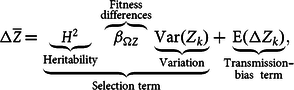 $$\matrix{ {{\rm{\Delta }}\overline Z} \, { = \underbrace {\underbrace {{H^2}}_{{\rm{Heritability}}}\overbrace {{\beta _{{\rm{\Omega }}Z}}}^{\scriptstyle \rm {Fitness} \atop \scriptstyle {\rm differences}}\underbrace {\rm{Var}\left( {\it {Z}_{\it{k}}} \right)}_{{\rm{Variation}}}}_{{\rm{Selection\;term}}} +\!\! \underbrace {\rm E\left( {{\rm{\Delta }}{\it{Z}_{\it k}}} \right)}_{\scriptstyle {\rm{Transmission}} {\hbox-}\atop \scriptstyle {\rm{bias\;\;term}} } \hskip -5pt,} \cr } $$
where
 ${\beta _{{\rm{\Omega }}Z}}$
is the linear regression coefficient of
${\beta _{{\rm{\Omega }}Z}}$
is the linear regression coefficient of
 ${\rm{\Omega }}$
on
${\rm{\Omega }}$
on
 $Z$
obtained from the least-squares method by transformation of
$Z$
obtained from the least-squares method by transformation of
 ${\rm{Cov}}\left( {{{\rm{\Omega }}_k},{Z_k}} \right)$
into
${\rm{Cov}}\left( {{{\rm{\Omega }}_k},{Z_k}} \right)$
into
 ${\beta _{{\rm{\Omega }}Z}}{\rm{Var}}\left( {{Z_k}} \right)$
(for more on this method, see Lynch and Walsh Reference Lynch and Walsh1998, chap. 3);
${\beta _{{\rm{\Omega }}Z}}{\rm{Var}}\left( {{Z_k}} \right)$
(for more on this method, see Lynch and Walsh Reference Lynch and Walsh1998, chap. 3);
 ${\rm{Var}}\left( {{Z_k}} \right)$
is the variance of
${\rm{Var}}\left( {{Z_k}} \right)$
is the variance of
 $Z$
; and
$Z$
; and
 ${H^2}$
represents the heritability of character
${H^2}$
represents the heritability of character
 $Z$
, which, again following the standard least-squares method, is the regression coefficient of average offspring character on parental character, which is defined as
$Z$
, which, again following the standard least-squares method, is the regression coefficient of average offspring character on parental character, which is defined as
 ${{{\rm{Cov}}\left( {\overline {Z{{\rm{'}}_k}} ,{Z_k}} \right)} \over {{\rm{Var}}\left( Z \right)}}$
 ${\rm{Cov}}\left( {{{\rm{\Omega }}_k},{Z_i}} \right)$
; and
${\rm{Cov}}\left( {{{\rm{\Omega }}_k},{Z_i}} \right)$
; and
 ${\rm{E}}\left( {{\rm{\Delta }}{Z_k}} \right)$
is the transmission bias.
Footnote 6
${\rm{E}}\left( {{\rm{\Delta }}{Z_k}} \right)$
is the transmission bias.
Footnote 6
Equation (2) connects to Lewontin’s conditions in the following way. The condition of variation is satisfied when
 ${\rm{Var}}\left( {{Z_k}} \right) \ne 0$
. The condition of fitness difference is satisfied when
${\rm{Var}}\left( {{Z_k}} \right) \ne 0$
. The condition of fitness difference is satisfied when
 ${\beta _{{\rm{\Omega }}Z}} \ne 0$
, assuming that relative growth can be associated with fitness (
${\beta _{{\rm{\Omega }}Z}} \ne 0$
, assuming that relative growth can be associated with fitness (
 ${\rm{\Omega }}$
). Finally, the condition of heredity is satisfied if
${\rm{\Omega }}$
). Finally, the condition of heredity is satisfied if
 ${H^2} \ne 0$
(see Okasha Reference Okasha2006, chap. 1). If any of these terms is
${H^2} \ne 0$
(see Okasha Reference Okasha2006, chap. 1). If any of these terms is
 $0$
, ENS does not occur. Equation (2) also contains a transmission-bias term that corresponds to evolutionary change due to evolutionary processes that are different from natural selection. Lewontin’s conditions do not cover such processes; thus, in some sense, the Price equation is more general than the three conditions.
Footnote 7
$0$
, ENS does not occur. Equation (2) also contains a transmission-bias term that corresponds to evolutionary change due to evolutionary processes that are different from natural selection. Lewontin’s conditions do not cover such processes; thus, in some sense, the Price equation is more general than the three conditions.
Footnote 7
Although equations (1) and (2) are mathematically equivalent, we can see here that
 ${\rm{\Omega }}$
is not present in the transmission-bias term of equation (2). In consequence, the Lewontinized version separates the evolutionary change due to natural selection from that due to other evolutionary processes more “cleanly” than equation (1) does. Thus, when I refer to the Price equation in the remainder of the article, I will mean equation (2) or other forms derived directly from it.
${\rm{\Omega }}$
is not present in the transmission-bias term of equation (2). In consequence, the Lewontinized version separates the evolutionary change due to natural selection from that due to other evolutionary processes more “cleanly” than equation (1) does. Thus, when I refer to the Price equation in the remainder of the article, I will mean equation (2) or other forms derived directly from it.
One notable aspect of the different partitionings of the Price equation, and equation (2) in particular, is that they can be deployed recursively, assuming that (1) the entities of the same class as
 $k$
can be decomposed into nonoverlapping subentities, and (2) the character
$k$
can be decomposed into nonoverlapping subentities, and (2) the character
 $Z$
of the
$Z$
of the
 $k$
th entity and entities of its class is a statistical aggregate of the character of the subentities that compose them. To deploy the Price equation recursively, notice that in the transmission-bias term of equation (2), we have the term
$k$
th entity and entities of its class is a statistical aggregate of the character of the subentities that compose them. To deploy the Price equation recursively, notice that in the transmission-bias term of equation (2), we have the term
 ${\rm{\Delta }}{Z_k}$
. This term is similar to
${\rm{\Delta }}{Z_k}$
. This term is similar to
 ${\rm{\Delta }}\overline Z$
. The only difference between the two terms is that the change in character in
${\rm{\Delta }}\overline Z$
. The only difference between the two terms is that the change in character in
 ${\rm{\Delta }}\overline Z$
refers to the population, whereas it refers to the
${\rm{\Delta }}\overline Z$
refers to the population, whereas it refers to the
 $k$
th entity in
$k$
th entity in
 ${\rm{\Delta }}{Z_k}$
. If we assume that each entity of the same class as
${\rm{\Delta }}{Z_k}$
. If we assume that each entity of the same class as
 $k$
is made of
$k$
is made of
 $n$
subentities,
Footnote 8
we can define
$n$
subentities,
Footnote 8
we can define
 ${z_{kj}}$
and
${z_{kj}}$
and
 ${\omega _{kj}}$
as the character and relative growth,
Footnote 9
respectively, of the
${\omega _{kj}}$
as the character and relative growth,
Footnote 9
respectively, of the
 $j$
th subentity within the
$j$
th subentity within the
 $k$
th entity and rewrite
$k$
th entity and rewrite
 ${\rm{\Delta }}{Z_k}$
as:
${\rm{\Delta }}{Z_k}$
as:
 $$\begin{equation}\begin{split}
\Delta Z_k&=h_k^2\operatorname{cov_k}(\omega_{kj},z_{kj})+\operatorname{E_k}(\Delta z_{kj})\\
&= \underbrace{\underbrace{h_k^2}_{{\substack{\text{Heritability}\\ \text{within the}\\ \text{$k$th entity} }}} \overbrace{\beta_{\omega z}}^{{\substack{\text{Fitness differences} \\ \text{within the $k$th entity}}}} \underbrace{\operatorname{var_k}(z_{kj})}_{{\substack{\text{Variation}\\ \text{within the} \\ \text{$k$th entity}}}}}_{\substack{\text{Selection term}\\ \text{within the kth entity}}} +\overbrace{\operatorname{E_k}(\Delta z_{kj})}^{{\substack{\text{Transmission-}\\ \text{bias term within} \\ \text{the $k$th entity}}}},\\
\end{split}
\end{equation}$$
$$\begin{equation}\begin{split}
\Delta Z_k&=h_k^2\operatorname{cov_k}(\omega_{kj},z_{kj})+\operatorname{E_k}(\Delta z_{kj})\\
&= \underbrace{\underbrace{h_k^2}_{{\substack{\text{Heritability}\\ \text{within the}\\ \text{$k$th entity} }}} \overbrace{\beta_{\omega z}}^{{\substack{\text{Fitness differences} \\ \text{within the $k$th entity}}}} \underbrace{\operatorname{var_k}(z_{kj})}_{{\substack{\text{Variation}\\ \text{within the} \\ \text{$k$th entity}}}}}_{\substack{\text{Selection term}\\ \text{within the kth entity}}} +\overbrace{\operatorname{E_k}(\Delta z_{kj})}^{{\substack{\text{Transmission-}\\ \text{bias term within} \\ \text{the $k$th entity}}}},\\
\end{split}
\end{equation}$$
where
 ${\rm{Co}}{{\rm{v}}_{\rm{k}}}\left( {{\omega _{kj}}} ,{z_{kj}}\right)$
represents the covariance between
${\rm{Co}}{{\rm{v}}_{\rm{k}}}\left( {{\omega _{kj}}} ,{z_{kj}}\right)$
represents the covariance between
 $z$
and
$z$
and
 $\omega $
within
$\omega $
within
 $k$
;
$k$
;
 ${\rm{Va}}{{\rm{r}}_{\rm{k}}}\left( {{z_{kj}}} \right)$
represents the variance of
${\rm{Va}}{{\rm{r}}_{\rm{k}}}\left( {{z_{kj}}} \right)$
represents the variance of
 $z$
within
$z$
within
 $k$
;
$k$
;
 $h_k^2$
represents the heritability of character
$h_k^2$
represents the heritability of character
 $z$
within entity
$z$
within entity
 $k$
, which is defined as
$k$
, which is defined as
 ${{{\rm{Co}}{{\rm{v}}_{\rm{k}}}\left( {\overline {z{{\rm{'}}_{\hskip -1.5pt kj}}} ,{z_{kj}}} \right)} \over {{\rm{Va}}{{\rm{r}}_{\rm{k}}}\left( {\overline z} \right)}}$
, where
${{{\rm{Co}}{{\rm{v}}_{\rm{k}}}\left( {\overline {z{{\rm{'}}_{\hskip -1.5pt kj}}} ,{z_{kj}}} \right)} \over {{\rm{Va}}{{\rm{r}}_{\rm{k}}}\left( {\overline z} \right)}}$
, where
 $\overline {z{{\rm{'}}_{\hskip -2pt kj}}} $
is the average character value of the offspring of the
$\overline {z{{\rm{'}}_{\hskip -2pt kj}}} $
is the average character value of the offspring of the
 $j$
th subentity within
$j$
th subentity within
 $k$
; and finally,
$k$
; and finally,
 ${\rm{E_k}}\left( {{\rm{\Delta }}{z_{kj}}} \right)$
represents the transmission bias within
${\rm{E_k}}\left( {{\rm{\Delta }}{z_{kj}}} \right)$
represents the transmission bias within
 $k$
. By the standard least-squares method, we can transform
$k$
. By the standard least-squares method, we can transform
 ${\rm{Co}}{{\rm{v}}_{\rm{k}}}\left( {{\omega _{kj}},{z_{kj}}} \right)$
to
${\rm{Co}}{{\rm{v}}_{\rm{k}}}\left( {{\omega _{kj}},{z_{kj}}} \right)$
to
 ${\beta _{k\omega Z}}{\rm{Var}}\left( {{z_k}} \right)$
, where
${\beta _{k\omega Z}}{\rm{Var}}\left( {{z_k}} \right)$
, where
 ${\beta _{k\omega z}}$
is the linear regression coefficient of the relative growth of subentities on the character
${\beta _{k\omega z}}$
is the linear regression coefficient of the relative growth of subentities on the character
 $Z$
within entity
$Z$
within entity
 $k$
.
$k$
.
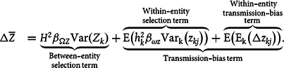
With equation (3) in place, we can plug it into equation (2). This leads to the following: Footnote 10
 $$\begin{equation}
\begin{split}
\Delta \overline{Z}&=\underbrace{H^2 \beta_{\Omega Z}\operatorname{var}(Z_k)}_{{\substack{\text{Between-entity}\\ \text{selection term}}}}+\underbrace{\overbrace{\operatorname{E}(h_k^2 \beta_{\omega z} \operatorname{var_k}(z_{kj}))}^{{\substack{\text{Within-entity}\\ \text{selection term} }}} + \overbrace{\operatorname{E}(\operatorname{E_k}(\Delta z_{kj}))}^{{\substack{\text{Within-entity}\\ \text{transmission-bias} \\ \text{term}}}}}_{{\substack{\text{Transmission-bias term}}}}.
\end{split}
\end{equation}$$
$$\begin{equation}
\begin{split}
\Delta \overline{Z}&=\underbrace{H^2 \beta_{\Omega Z}\operatorname{var}(Z_k)}_{{\substack{\text{Between-entity}\\ \text{selection term}}}}+\underbrace{\overbrace{\operatorname{E}(h_k^2 \beta_{\omega z} \operatorname{var_k}(z_{kj}))}^{{\substack{\text{Within-entity}\\ \text{selection term} }}} + \overbrace{\operatorname{E}(\operatorname{E_k}(\Delta z_{kj}))}^{{\substack{\text{Within-entity}\\ \text{transmission-bias} \\ \text{term}}}}}_{{\substack{\text{Transmission-bias term}}}}.
\end{split}
\end{equation}$$
This recursive process can be repeated indefinitely unless the subentities at a lower level cannot be decomposed any further or reproduced faithfully. This is so because a non-nil transmission bias at any level involves a change in character that can potentially be decomposed further into a selection term and transmission-bias term one level below. For instance, assuming the
 $j$
th subentity in the
$j$
th subentity in the
 $k$
th entity is itself multipartite,
$k$
th entity is itself multipartite,
 ${\rm{\Delta }}{z_{kj}}$
could be decomposed further into a selection term and a transmission-bias term within the subentities of the same class as
${\rm{\Delta }}{z_{kj}}$
could be decomposed further into a selection term and a transmission-bias term within the subentities of the same class as
 $j$
. Equation (4) is a multilevel version of the Price equation, the latter of which was proposed by Price (Reference Price1972) and one of the main tools used to restore some respect for the idea of group selection (Hamilton Reference Hamilton and Fox1975; Sober and Wilson Reference Sober and Sloan Wilson1998; Okasha Reference Okasha2006).
$j$
. Equation (4) is a multilevel version of the Price equation, the latter of which was proposed by Price (Reference Price1972) and one of the main tools used to restore some respect for the idea of group selection (Hamilton Reference Hamilton and Fox1975; Sober and Wilson Reference Sober and Sloan Wilson1998; Okasha Reference Okasha2006).
An important remark to make at this point is that equation (2) and equation (4) are both correct following the definitions of the terms provided. It does not make sense to claim that one is the correct interpretation. They are simply two alternative perspectives on the same evolutionary change. However, this calls into question the nature of selection processes when compared to other evolutionary processes. In particular, the comparison between the two equations shows that from one perspective, what is considered a transmission bias could equally be considered as selection processes occurring within entities. One might find it convenient to use one description rather than the other, but such pragmatic decisions are not based on a factual distinction. This last remark will prove crucial in the context of Darwinizing Gaia.
3. Generalizing the Price equation for ENS sans reproduction
In the previous section, I mentioned that a common assumption made when deriving the Price equation is that the time period
 ${\rm{\Delta }}Z$
is two generations. However, another notable aspect of the Price equation is that it can refer to any time period.
Footnote 11
This means that one can deploy the Price equation over periods of time shorter than a single generation. More generally, all the equation requires to be used is a mapping between two sets. This means that the scope of the equation is much more general and can apply to any situation of change, a point made by Price himself, who aimed to propose a general theory of selection (see Price Reference Price1995). A minimal Darwinian interpretation of the equation is that the elements of the sets represent individuals and that the sets represent a population at two different points in time. However, whether one considers situations in which there is no reproduction as representing genuine cases of ENS cannot come from the Price equation alone because it is a mathematical identity devoid of any empirical content. In other words, the abstractness of the equation makes it a versatile tool, but the interpretation of its terms is not contained in the equation itself.
${\rm{\Delta }}Z$
is two generations. However, another notable aspect of the Price equation is that it can refer to any time period.
Footnote 11
This means that one can deploy the Price equation over periods of time shorter than a single generation. More generally, all the equation requires to be used is a mapping between two sets. This means that the scope of the equation is much more general and can apply to any situation of change, a point made by Price himself, who aimed to propose a general theory of selection (see Price Reference Price1995). A minimal Darwinian interpretation of the equation is that the elements of the sets represent individuals and that the sets represent a population at two different points in time. However, whether one considers situations in which there is no reproduction as representing genuine cases of ENS cannot come from the Price equation alone because it is a mathematical identity devoid of any empirical content. In other words, the abstractness of the equation makes it a versatile tool, but the interpretation of its terms is not contained in the equation itself.
Once one comes to terms with this point, it becomes clear that equation (2) can be regarded as much more general than typically considered and applied to situations where there is no reproduction. However, whether one should associate these more general terms with ENS could be disputed. Although some will regard situations where there is no reproduction as merely marginal cases of ENS (see Godfrey-Smith Reference Godfrey-Smith2009), if at all, there are numerous reasons to regard the requirement of reproduction for ENS to occur as problematic, as highlighted by numerous authors (see Van Valen Reference Van Valen1976; Bouchard Reference Bouchard2008, Reference Bouchard2011; Bourrat Reference Bourrat2014, Reference Bourrat2015, Reference Bourrat2021b; Papale Reference Papale2021; Takacs and Bourrat Reference Takacs and Bourrat2022). If one is convinced by these arguments (as I am, and which, for lack of space, I will not rehearse here), the terms
 ${\rm{\Omega }}$
,
${\rm{\Omega }}$
,
 ${H^2}$
, and
${H^2}$
, and
 ${\rm E}\left( {{\rm{\Delta }}{Z_k}} \right)$
can apply to situations involving no reproduction.
${\rm E}\left( {{\rm{\Delta }}{Z_k}} \right)$
can apply to situations involving no reproduction.
4. Returning to Gaia
In the preceding sections, I presented a conceptual apparatus that I will now deploy to demonstrate that the idea of Gaia can be understood squarely within a Darwinian framework. To do so, I show that one can provide equivalent Price formulations of Gaia’s directional change for a given character at different levels of description—one at the global level and some other descriptions at lower levels. At the higher (global) level of description, the evolutionary change is fully described in terms of transmission bias, understood here as persistence; however, under alternative descriptions, this transmission bias can be explained in terms of selection, rendering the change observed de facto Darwinian.
To begin, recall that in the Gaia hypothesis, Gaia is a single entity. What are the implications of this in equations (2) and (4)? Let us assume that Gaia represents a population comprising a single entity and that
 $Z$
is any trait that can be measured at any biological scale (e.g., albedo), in a similar fashion as the Daisyworld model discussed earlier. Because Gaia is a single entity, there is no variation upon which natural selection can work. Formally, the variance term,
$Z$
is any trait that can be measured at any biological scale (e.g., albedo), in a similar fashion as the Daisyworld model discussed earlier. Because Gaia is a single entity, there is no variation upon which natural selection can work. Formally, the variance term,
 ${\rm{Var}}\left( {{Z_k}} \right)$
, is nil because the variance of a random variable that can only take a single value is nil.
Footnote 12
This means that equation (2), under those assumptions, becomes
${\rm{Var}}\left( {{Z_k}} \right)$
, is nil because the variance of a random variable that can only take a single value is nil.
Footnote 12
This means that equation (2), under those assumptions, becomes
 $$\matrix{ {{\rm{\Delta }}\overline Z} \;{ = {H^2}{\beta _{{\rm{\Omega }}Z}} \times 0 + {\rm{E}}\left( {{\rm{\Delta }}{Z_k}} \right)} \hfill \cr {} \hfill \!\!\!\!{ = {\rm{E}}\left( {{\rm{\Delta }}{Z_k}} \right) = {\rm{\Delta }}{Z_k},} \hfill \cr } $$
where
 $k$
refers to the sole entity of the population—namely, Gaia.
$k$
refers to the sole entity of the population—namely, Gaia.
This equation shows that in a situation where there is a single entity, evolutionary change (
 ${\rm{\Delta }}\overline Z$
) can only be due to transmission bias—understood, in this case, as the same entity changing over time. In and of itself, this description seems to vindicate the idea that natural selection ought to be divorced from the Gaia hypothesis because the term related to natural selection is nil.
${\rm{\Delta }}\overline Z$
) can only be due to transmission bias—understood, in this case, as the same entity changing over time. In and of itself, this description seems to vindicate the idea that natural selection ought to be divorced from the Gaia hypothesis because the term related to natural selection is nil.
However, by simply changing the level at which the Gaia system is described, such as the ecosystem level or the individual organism level, which both correspond to descriptions with some valid empirical justifications, this conclusion is not required to hold. Suppose, as in figure 1a, that a trait (albedo) of the Gaia system is changing over time from a value of
 $0$
(black) to
$0$
(black) to
 $1$
(white), with different shades of gray in between. In this example, the change occurs over four periods of time, from
$1$
(white), with different shades of gray in between. In this example, the change occurs over four periods of time, from
 ${t_1}$
to
${t_1}$
to
 ${t_5}$
, at a constant rate. This corresponds to the situation where the transmission bias (
${t_5}$
, at a constant rate. This corresponds to the situation where the transmission bias (
 ${\rm{\Delta }}{Z_k}$
) of the system, which fully explains the change of the system (
${\rm{\Delta }}{Z_k}$
) of the system, which fully explains the change of the system (
 ${\rm{\Delta }}\overline Z$
), using equation (2), changes from
${\rm{\Delta }}\overline Z$
), using equation (2), changes from
 $0$
to
$0$
to
 $0.25$
between
$0.25$
between
 ${t_1}$
and
${t_1}$
and
 ${t_2}$
, from
${t_2}$
, from
 $0.25$
to
$0.25$
to
 $0.5$
between
$0.5$
between
 ${t_2}$
and
${t_2}$
and
 ${t_3}$
, from
${t_3}$
, from
 $0.5$
to
$0.5$
to
 $0.75$
between
$0.75$
between
 ${t_3}$
and
${t_3}$
and
 ${t_4}$
, and from
${t_4}$
, and from
 $0.75$
to
$0.75$
to
 $1$
between
$1$
between
 ${t_4}$
and
${t_4}$
and
 ${t_5}$
.
${t_5}$
.

Figure 1. Three equivalent perspectives on the evolution of a system over four periods of time for a trait. (a) The global system’s character change is a result of “mutations” (i.e., a transmission bias) from 0 (black) to 1 (white), with an increment of 0.25 over each period of time. (b) The change is explained by processes occurring at a lower level rather than the global system—namely, the selection of ecosystems with a higher character value (from t 2 to t 3) and the “mutation” of ecosystems (from t 1 to t 2, t 3 to t 4, and t 4 to t 5). (c) The change is explained by processes occurring at a lower level rather than at the ecosystem level—namely, by selection between individual organisms (from t 2 to t 3 and t 4 to t 5) and the mutation of individuals (from t 1 to t 2 and t 3 to t 4). We assume here that each time period represents an individual-level generation and that generations are discrete.
Now, suppose that the Gaia system comprises subentities, namely, ecosystems—a perfectly plausible assumption—with the possibility for them to have different levels of albedo, as in figure 1b. Further, assume that ecosystem albedo levels sum up to the level of albedo of the Gaia system—another plausible assumption. Under these conditions, at least part of the transmission bias between two times might correspond to selection at this lower level of description. This is the case in figure 1b and can be seen by comparing the evolutionary change from
 ${t_1}$
to
${t_1}$
to
 ${t_2}$
and from
${t_2}$
and from
 ${t_2}$
to
${t_2}$
to
 ${t_3}$
. Starting from
${t_3}$
. Starting from
 ${t_1}$
to
${t_1}$
to
 ${t_2}$
, assuming the Gaia system can be decomposed into four ecosystems of equal size (this assumption is, again, made for simplicity), one of the ecosystems with the value
${t_2}$
, assuming the Gaia system can be decomposed into four ecosystems of equal size (this assumption is, again, made for simplicity), one of the ecosystems with the value
 $0$
might “mutate” and have the value
$0$
might “mutate” and have the value
 $1$
at
$1$
at
 ${t_2}$
. The transmission bias at the global level would here be explained fully by a transmission bias at the lower level. However, between
${t_2}$
. The transmission bias at the global level would here be explained fully by a transmission bias at the lower level. However, between
 ${t_2}$
and
${t_2}$
and
 ${t_3}$
, we could assume that there is an advantage for ecosystems with a high level of albedo; thus, they are more likely to replace (by differential growth) ecosystems with lower levels of albedo. This could be due to, for instance, the fact that ecosystems with a high level of albedo happen to also thrive in environments with a lower temperature than ecosystems with a lower albedo level. In figure 1, this is represented by a blue arrow that symbolizes growth or reproduction and a red cross that symbolizes death or elimination. The change in the level of albedo at the global level due to transmission bias for a fully persisting entity would be explained fully as selection at the ecosystem level by the differential death and growth of the ecosystems composing Gaia, leading the entire system to be composed, at
${t_3}$
, we could assume that there is an advantage for ecosystems with a high level of albedo; thus, they are more likely to replace (by differential growth) ecosystems with lower levels of albedo. This could be due to, for instance, the fact that ecosystems with a high level of albedo happen to also thrive in environments with a lower temperature than ecosystems with a lower albedo level. In figure 1, this is represented by a blue arrow that symbolizes growth or reproduction and a red cross that symbolizes death or elimination. The change in the level of albedo at the global level due to transmission bias for a fully persisting entity would be explained fully as selection at the ecosystem level by the differential death and growth of the ecosystems composing Gaia, leading the entire system to be composed, at
 ${t_3}$
, of only two ecosystems rather than four. From
${t_3}$
, of only two ecosystems rather than four. From
 ${t_3}$
to
${t_3}$
to
 ${t_4}$
and
${t_4}$
and
 ${t_4}$
to
${t_4}$
to
 ${t_5}$
, the evolutionary change at the ecosystem-level description occurs by transmission bias only.
${t_5}$
, the evolutionary change at the ecosystem-level description occurs by transmission bias only.
Ecosystems are composed of individual organisms; thus, we can describe the Gaia system from yet another, lower perspective—namely, the individual organism level. From this third perspective, ecosystems are made up of two types of individuals (again, this assumption is made for simplicity), and the evolutionary change between the four periods of time between
 ${t_1}$
and
${t_1}$
and
 ${t_5}$
in figure 1c is explained by selection in the classic sense (i.e., by differential reproduction, rather than differential persistence and growth) and transmission bias. We assume here that individuals reproduce in discrete generations (with one generation being one of the four periods of time); generations have only two values,
${t_5}$
in figure 1c is explained by selection in the classic sense (i.e., by differential reproduction, rather than differential persistence and growth) and transmission bias. We assume here that individuals reproduce in discrete generations (with one generation being one of the four periods of time); generations have only two values,
 $0$
and
$0$
and
 $1$
(as in the original Daisyworld model); and reproduction can be imperfect. From this third perspective, the evolutionary change explained by a positive transmission bias from
$1$
(as in the original Daisyworld model); and reproduction can be imperfect. From this third perspective, the evolutionary change explained by a positive transmission bias from
 ${t_2}$
to
${t_2}$
to
 ${t_3}$
and
${t_3}$
and
 ${t_4}$
to
${t_4}$
to
 ${t_5}$
at the global level can be explained by selection at the individual organism level. We can also see that from
${t_5}$
at the global level can be explained by selection at the individual organism level. We can also see that from
 ${t_3}$
to
${t_3}$
to
 ${t_4}$
, what was explained as an evolutionary change due to transmission bias of the Gaia system (figure 1a) or of ecosystems (figure 1b) now becomes explained as a change due to a transmission bias at the individual organism level.
${t_4}$
, what was explained as an evolutionary change due to transmission bias of the Gaia system (figure 1a) or of ecosystems (figure 1b) now becomes explained as a change due to a transmission bias at the individual organism level.
More formally, the redescriptions of the evolutionary change due to the transmission bias at the global level (Gaia) in terms referring to ecosystems or individual organisms in the example presented in figure 1 can be performed by applying equation (2) recursively to equation (5). Thus, redescribing the global system from a lower level of description, we obtain:
 $${\rm{\Delta }}{Z_k} = h_k^2{\beta _{\omega z}}{\rm{Va}}{{\rm{r}}_{\rm{k}}}\left( {{z_{kj}}} \right) + {{\rm{E}}_{\rm{k}}}\left( {{\rm{\Delta }}{z_{kj}}} \right),$$
where
 $k$
refers to Gaia, and
$k$
refers to Gaia, and
 $j$
refers to an ecosystem (or alternatively, individual organism).
$j$
refers to an ecosystem (or alternatively, individual organism).
Between
 ${t_2}$
and
${t_2}$
and
 ${t_3}$
, there is no transmission bias of ecosystems—that is, when they persist and grow, their character does not change. Equation (6) becomes:
${t_3}$
, there is no transmission bias of ecosystems—that is, when they persist and grow, their character does not change. Equation (6) becomes:
 $${\rm{\Delta }}{Z_k} = h_k^2{\beta _{\omega z}}{\rm{Va}}{{\rm{r}}_{\rm{k}}}\left( {{z_{kj}}} \right).$$
Computing
 $h_k^2$
,
$h_k^2$
,
 ${\beta _{\omega z}}$
, and
${\beta _{\omega z}}$
, and
 ${\rm{Va}}{{\rm{r}}_{\rm{k}}}\left( {{z_{kj}}} \right)$
, using the values of
${\rm{Va}}{{\rm{r}}_{\rm{k}}}\left( {{z_{kj}}} \right)$
, using the values of
 $0$
,
$0$
,
 $1$
, and
$1$
, and
 $2$
for the relative growth of ecosystems going extinct, persisting, and growing, respectively (as shown in figure 1b), we find that the change due to selection is
$2$
for the relative growth of ecosystems going extinct, persisting, and growing, respectively (as shown in figure 1b), we find that the change due to selection is
 $0.25$
, as expected. Similarly, if we now take equation (6) and consider that subentities of the same class as
$0.25$
, as expected. Similarly, if we now take equation (6) and consider that subentities of the same class as
 $j$
do not refer to ecosystems but to individual organisms, and we apply this equation between
$j$
do not refer to ecosystems but to individual organisms, and we apply this equation between
 ${t_4}$
and
${t_4}$
and
 ${t_5}$
, we find the same result as previously. Namely, selection at the individual organism level is fully driving the evolutionary change observed between those two times—equation (6) reduces to equation (7)—which, again, is
${t_5}$
, we find the same result as previously. Namely, selection at the individual organism level is fully driving the evolutionary change observed between those two times—equation (6) reduces to equation (7)—which, again, is
 $0.25$
.
$0.25$
.
However, if we apply this equation at the individual organism level in situations where the change is due solely to transmission bias, as is the case between
 ${t_3}$
and
${t_3}$
and
 ${t_4}$
, the equation becomes:
${t_4}$
, the equation becomes:
 $${\rm{\Delta }}{Z_k} = {{\rm{E}}_{\rm{k}}}\left( {{\rm{\Delta }}{z_{kj}}} \right).$$
Once we compute the average of the eight individual transmission biases in our example, which amount to
 $0$
for six of them and
$0$
for six of them and
 $1$
for the two individuals with the character value of
$1$
for the two individuals with the character value of
 $0$
, we obtain
$0$
, we obtain
 ${\rm{\Delta }}{Z_k} = {2 \over 8} = 0.25$
, as expected.
${\rm{\Delta }}{Z_k} = {2 \over 8} = 0.25$
, as expected.
The simple example presented in this section could be compexified and applied to traits with covariation between them, as is done in quantitative genetics using variance and covariance matrices (see Roff Reference Roff1997).
5. Dispelling three objections
In the previous section, I showed, via deploying a multilevel version of the Price equation, that the evolution of the Gaia system is fully compatible with Darwinian principles, assuming that the lower-level entities composing the Gaia system are undergoing selection processes.
At that point, one might be convinced by the “in principle” argument but deny that lower entities (i.e., ecosystems or individual organisms belonging to different species) are in Darwinian competition. Classically, for two entities to be said to be in competition requires that they are in a common selective environment (Brandon Reference Brandon1990). One might wish to deny that two ecosystems or two individual organisms belonging to two species have a common selective environment. For instance, at first pass, it seems obvious that a terrestrial species cannot be in competition with an aquatic one. However, for these individuals to be seen as belonging to a common selective environment requires moving away from the classic framing for which the tools in evolutionary theory have been devised—namely, local populations over relatively short periods. Over longer periods at the global level, two separated and different ecosystems or two individuals belonging to two species living under two different sets of ecological conditions might be said to be in competition with one another for the free energy available on Earth. This was a hypothesis proposed by Van Valen (Reference Van Valen1976), who argued that energy control is the ultimate measure of fitness and could allow one to compare the fitness of different taxa. Notably, although often forgotten, this reasoning also formed the basis of his Red Queen hypothesis. Without having to agree with Van Valen’s proposal, a more general point stands: there is nothing intrinsic to evolutionary theory, especially once coupled with an ecological perspective, that forbids one from moving to a global scale and discussing a common selective environment where the features of this environment are global variables, such as the level of albedo on Earth, and a highly abstract concept of fitness. Footnote 13
A second objection to the analysis proposed here would consist of acknowledging that natural selection and adaptation can occur at levels below Gaia and that, as such, adapted entities exist at those lower levels, but also point out that it does not entail that the whole system exhibits adaptations at that level. I see no particular flaw with this line of reasoning; however, I believe that the claim that Earth is an adapted system can be understood in a legitimately different way from the one just presented. Namely, the question asked might be whether the change in the trait under consideration at the global level is the outcome of natural selection, even when looked at from the lower levels. The legitimacy of this question is warranted by the fact that the compatibility of Darwinism and Gaia has been challenged in the context where most protagonists of the debate start from the premise that if there are selection processes, they occur at a level below Gaia. Recall, for instance, from the introduction, that the model quickly dismissed by Dawkins only involves competition between entities below the global system.
To see how different scenarios could lead to different answers about whether Gaia is adapted under this different sense, recall that in figure 1, I presented a setting in which some within-entity selection occurs at both the ecosystem and individual levels between
 ${t_1}$
and
${t_1}$
and
 ${t_5}$
. However, I could equally well have presented a different example where the change observed at the global level yields no selection component at any level and over any period of time. Formally, using equation (6), and assuming that entities at the same level as
${t_5}$
. However, I could equally well have presented a different example where the change observed at the global level yields no selection component at any level and over any period of time. Formally, using equation (6), and assuming that entities at the same level as
 $j$
represent ecosystems, this would mean that we would find no selection between ecosystems, as well as a transmission bias at the level of ecosystems different from
$j$
represent ecosystems, this would mean that we would find no selection between ecosystems, as well as a transmission bias at the level of ecosystems different from
 $0$
. This would be equivalent to the situation described between
$0$
. This would be equivalent to the situation described between
 ${t_3}$
and
${t_3}$
and
 ${t_4}$
, so equation (6) reduces to equation (8), but would apply here to all periods of time. In addition, further decomposing the transmission bias of equation (8) into a within-ecosystem selection term and a within-ecosystem transmission-bias term, we would find that the within-ecosystem selection term is nil no matter how low the level at which we decompose this term. In such a situation, the claim that Gaia exhibits ENS or adaptation would be false, irrespective of whether one considers that selection and adaptation refer to a particular level.
${t_4}$
, so equation (6) reduces to equation (8), but would apply here to all periods of time. In addition, further decomposing the transmission bias of equation (8) into a within-ecosystem selection term and a within-ecosystem transmission-bias term, we would find that the within-ecosystem selection term is nil no matter how low the level at which we decompose this term. In such a situation, the claim that Gaia exhibits ENS or adaptation would be false, irrespective of whether one considers that selection and adaptation refer to a particular level.
Note, importantly, that finding a nil within-ecosystem selection term would not necessarily mean that no selection occurs between subentities, such as individuals, within an ecosystem. It would only imply that the average of the selection processes occurring within ecosystems is nil. Specifically, it could very well be the case that for every change due to selection within one ecosystem, there is an opposite change due to selection occurring in another ecosystem, leading ultimately to a nil expected value. This point is crucial—the presence of natural selection at a local level does not necessarily translate into a change and, consequently, adaptation at the global level.
A third objection to the proposal of the compatibility of Gaia with a Darwinian framework that could be characterized from a Pricean perspective echoes Dawkins’s worry that seeing Gaia as the result of a selection process occurring at the ecosystem level has the same problems as group selection—namely, that free riders can invade the group or, in this instance, the whole system and cause its demise. This problem is an instance of the tragedy of the commons (Hardin Reference Hardin1968). How should we address it?
From the Price equation alone and the arguments I have developed, we only have an argument that, fundamentally, the Gaia system can be regarded from different perspectives that are equivalent in their evolutionary outcome and that, under some perspectives, it would be legitimate to see some global traits as resulting from changes due to natural selection. This shows that natural selection and a single system evolving are, in principle, compatible with one another. Nonetheless, it does not explain why the global system is sustainable or, in other words, how a tragedy of the commons can be avoided. Although answering this question is beyond the purview of a Pricean analysis, it is important to address it to produce a complete Darwinian explanation.
In the albedo example presented earlier, assuming it follows the same dynamics as the original Daisyworld model, a negative feedback between albedo and temperature exists, so that if albedo increases, the black type will be favored, whereas the contrary is true when albedo decreases. However, the direction of the feedback between albedo and one of its by-products (changing the temperature of the system) has been stipulated without any principled justification. What would happen if the feedback, instead of being negative, was positive, or if one type could free ride and grow without needing the other type? Both cases would soon lead to the elimination of one of the two types—as shown, for instance, in some versions of the Daisyworld model where black daisies can produce white clouds and free ride on the white daisies, which become extinct (for details, see Lenton and Watson Reference Lenton and Watson2011, 123).
Let us suppose now that there are vital interactions for the maintenance of the whole system between the different types of subentities, so that if one type goes extinct, sooner or later, the whole system collapses. In the case of the Daisyworld model, this would mean that the two types must be present on the planet. A scenario where one type can invade the population—due to the existence of either positive feedback or free riding, as we have seen—represents, prima facie, a real threat to the hypothesis of the compatibility between Gaia and Darwinism. The alternative here would be to explain the persistence of the system by chance alone—the antithesis of the Gaia hypothesis. Fortunately, there are several important reasons to doubt that such scenarios are, in reality, likely. I will now present these, relying primarily on the work of Lenton and Watson (Reference Lenton and Watson2011) and Lenton et al. (Reference Lenton, Daines, Dyke, Nicholson, Wilkinson and Williams2018), who have spent years and sometimes—for some of the authors involved—decades refining their views.
First, let us note that one key assumption for the collapse-of-the-system argument to work, either through free riding or by positive feedback, is that the effects on the system coming from the by-product or the evolutionary strategy to outcompete other types, respectively, are globally negative. In cases with two types and a single regulatory mechanism for a variable, a collapse of the system is not difficult to imagine. However, it is more difficult to conceive when more types are present and the system is highly heterogeneous. With environmental heterogeneity, it is reasonable to suppose that there is more than one regulatory mechanism for a single variable. Concretely, albedo is not the only way to cool down or warm up the planet. Other factors resulting from the system activities can play a role, such as the production of greenhouse gases. There are also different ways to affect the albedo of the system, as illustrated by the example of white clouds produced by the black daisies. Environmental heterogeneity—which could be seen as heterogeneous patches—also implies different traits for the subentities between different parts of the global environment.
In situations of high heterogeneity in both the subentities composing the biosphere and the environment, a global collapse of the system could nonetheless occur, in principle, for two reasons: either as a result of global free riding or as a result of positive feedback affecting one or more global variables vital for the whole system. I discuss these in turn. First, in the case of free riding, we would need to assume a free rider that is so adaptable that it can invade all ecological niches of the system before the patches on which it free rides collapse. It is very difficult to imagine that such a species of free rider exists. Hamilton (Reference Hamilton1995) considers that the only such “Genghis Khan” species is us. But even in this instance, it is hard to conceive that humanity could destroy every ecosystem of the planet before this leads to our own extinction and that of many other species along the way. Even so, this would probably not lead to an absolute collapse of the system—only perhaps to a very different Gaia as we know it. Consequently, the hypothesis of a global free rider does not represent a real threat to the Gaia hypothesis as I have formulated it.
The case of positive feedback is different. For a global collapse to occur, we would need to assume that the by-product affects all parts of the system negatively and that the system has no potential for adaptation. That means an impossibility for local—that is, within a patch—adaptive responses to be selected or for the successful patches to take over the ones that collapsed. In cases where the negative effects only diffuse locally—perhaps less locally than neighbor patches but not globally—and occur after short periods following the activities that produced them, they will primarily affect the patches that produced them, ultimately leading to their demise. Following their demise, neighbor patches that do not produce the negative effects will colonize the empty patches, so global collapse will not occur.
However, the matter is different for variables that either have a global impact (which could result from a local impact that lasts for a very long time) or have negative effects that only appear long after their cause(s), which all parts of the system could have produced. Lenton et al. (Reference Lenton, Daines, Dyke, Nicholson, Wilkinson and Williams2018, 635) present key Earth system variables that satisfy these properties. In such situations, a global (or nearly global) collapse is possible, and this should be addressed if the Gaia hypothesis is to be made compatible with a Darwinian framework. As we will now see, Lenton and his colleagues have done precisely so with what they call sequential selection (Lenton et al. Reference Lenton, Daines, Dyke, Nicholson, Wilkinson and Williams2018; Lenton et al. Reference Lenton, Kohler, Marquet, Boyle, Crucifix, Wilkinson and Scheffer.2021).
To explain why global variables or variables with delayed effects are regulated as if they were the product of natural selection, Lenton et al. (Reference Lenton, Daines, Dyke, Nicholson, Wilkinson and Williams2018) propose a review of the literature on what they call sequential selection (for a convergent idea, see also Doolittle Reference Doolittle2014). Sequential selection, they argue, bears some similarity to the process of natural selection as we know it. Applied to Gaia, it works as follows. Once life has occurred, if a newly produced global system collapses or nearly so, but each time this occurs, a new system is rebuilt, after sufficient time, it is likely that the observed system is observed because it has properties that helped it persist. This process is, in some sense, equivalent to (but slower than) starting with a population of differential persisting entities and evolving it. Such a process of sequential selection occurring early in the history of life for global variables combined with the Darwinian mechanisms discussed earlier could explain why the biosphere appears to have regulatory mechanisms that constitute adaptations.
Further, one possible refinement of the sequential selection model is that even in a case of near collapse, either some species themselves or some parts of the environment modified by the biotic activities are reutilized in the next iteration of the system (for developments of this idea, see Arthur and Nicholson Reference Arthur and Nicholson2022, Reference Arthur and Nicholson2023). In both cases, this constitutes a form of inheritance or memory that would make sequential selection a form of selection that leads to cumulative evolution. All we would need to assume for this form of selection to increase the stability of the system over time is that the stability of the system parts aggregates into global stability. Under this assumption, combining different parts of the system that are stable, on average, would lead to a more stable global system in the next iteration than if the parts were less stable. Whether this assumption is verified for at least some global traits would need to be tested, but if it were the case, this would render the model one step closer to a Darwinian one.
6. Conclusion
In this article, I argued formally, using the Price equation, that the transformational evolution of the Gaia system, using Lewontin’s (Reference Lewontin1983) terminology, can be recast in terms of variational evolution due to natural selection at lower levels. Going beyond what a Pricean analysis can do, I argued (following recent work) that a Darwinian approach can make the regulation of the system of the whole planet Earth more likely than what would be expected by pure luck. Thus, changes or lack thereof of the whole system in response to environmental changes need not be interpreted teleologically or mysteriously—they can be understood, at least theoretically, as the outcome of selection processes occurring between the entities composing the system over much longer timescales than the timescales classically considered in evolutionary theory. When describing this system from lower levels over such timescales, populations (whether at a time or sequentially), variation, fitness differences, and inheritance all arise. Therefore, concerns that the Gaia system is overly teleological and incompatible with a Darwinian view should be laid to rest.
Acknowledgments
I thank Guilhem Doulcier, William Godsoe, and three anonymous reviewers for their comments on previous versions of this article. I gratefully acknowledge the financial support of the John Templeton Foundation (No. 62220). The opinions expressed in this article are those of the authors and not those of the John Templeton Foundation. This research was also supported under Australian Research Council’s Discovery Projects funding scheme (Project Number DE210100303).


 Open access