


1. Introduction
What concepts are essential to the proof of a given statement? This is a fundamental and long-debated question in logic since the time of Leibniz, Kant, and Frege, when a broad notion of analytic proof was formulated to mean truth by conceptual containments, or purity of method in mathematical arguments.
The familiar Hilbert-style proof systems are excellent for many purposes including defining a logic and a notion of proof. However they offer few insight concerning analyticity because of their reliance on the inference rule of modus ponens. The issue is that the conclusion B of modus ponens may be quite unrelated to the A that occurs in its premises
 $A\rightarrow B$
and A. In 1935, Gentzen [Reference Gentzen and Szabo20] showed how to address this weakness of the Hilbert systems by placing the logical language within a meta-logical (structural) language. Specifically, he introduced a new type of proof system called the sequent calculus built from sequents
$A\rightarrow B$
and A. In 1935, Gentzen [Reference Gentzen and Szabo20] showed how to address this weakness of the Hilbert systems by placing the logical language within a meta-logical (structural) language. Specifically, he introduced a new type of proof system called the sequent calculus built from sequents
 $\Gamma \Rightarrow \Delta $
where
$\Gamma \Rightarrow \Delta $
where
 $\Gamma $
and
$\Gamma $
and
 $\Delta $
are lists/multisets of logical formulas. Enriching the logical language with a structural language enabled him to state and prove the famous cut-elimination theorem—this is a constructive procedure that eliminates all applications of the cut rule from a given proof. The cut rule is a generalisation of modus ponens and it is the only non-analytic rule in the classical and intuitionistic sequent calculi. So from cut-elimination it follows that every provable formula has a proof respecting the subformula property (i.e., every formula in the proof is a subformula of the theorem). Gentzen later used this property to give a proof of the consistency of arithmetic. This cemented the significance of the sequent calculus, and analyticity came to be seen as near-synonymous with the subformula property.
$\Delta $
are lists/multisets of logical formulas. Enriching the logical language with a structural language enabled him to state and prove the famous cut-elimination theorem—this is a constructive procedure that eliminates all applications of the cut rule from a given proof. The cut rule is a generalisation of modus ponens and it is the only non-analytic rule in the classical and intuitionistic sequent calculi. So from cut-elimination it follows that every provable formula has a proof respecting the subformula property (i.e., every formula in the proof is a subformula of the theorem). Gentzen later used this property to give a proof of the consistency of arithmetic. This cemented the significance of the sequent calculus, and analyticity came to be seen as near-synonymous with the subformula property.
The decades following Gentzen’s work saw an explosion of results establishing the subformula property via cut-elimination for sequent calculi for various logics. The subformula property is a significant restriction on the proof search space which can be exploited to establish metalogical results (e.g., consistency, decidability, complexity, interpolation, and disjunction properties) and for automated reasoning. Nevertheless, already from the 1960s it was observed (for example, Mints [Reference Mints36]) that the formalism of the sequent calculus was not expressive enough to provide the subformula property for most logics of interest. The response of the structural proof theory community was to obtain the subformula property by developing new exotic proof formalisms (e.g., hypersequent, bunched, nested sequent, display, labelled calculi, tree-hypersequent, and many more) that further extend the structural language of the sequent calculus.
Introduced independently by Mints [Reference Mints36], Pottinger [Reference Pottinger38], and Avron [Reference Avron2], the hypersequent calculus is one of the most successful such formalisms. A hypersequent goes just one step further in the sense that it is a multiset of Gentzen’s sequents, denoted as
 $\Gamma _1 \Rightarrow \Delta _1 \mid \dots \mid \Gamma _n \Rightarrow \Delta _n$
. Hypersequent calculi with the subformula property have been presented for many non-classical logics that could not be provided this property in the sequent calculus. Especially noteworthy are the uniform and modular extensions of base systems for commutative substructural logics [Reference Ciabattoni, Galatos and Terui12] and modal logics [Reference Kurokawa, Nakano, Satoh and Bekki28, Reference Lahav29, Reference Lellmann31].
$\Gamma _1 \Rightarrow \Delta _1 \mid \dots \mid \Gamma _n \Rightarrow \Delta _n$
. Hypersequent calculi with the subformula property have been presented for many non-classical logics that could not be provided this property in the sequent calculus. Especially noteworthy are the uniform and modular extensions of base systems for commutative substructural logics [Reference Ciabattoni, Galatos and Terui12] and modal logics [Reference Kurokawa, Nakano, Satoh and Bekki28, Reference Lahav29, Reference Lellmann31].
However, the price to be paid for moving to an exotic proof formalism—even in the simple case of hypersequents—is having to tame its richer structural language in order to use the proof calculus to prove metalogical results.
Rather than privileging the subformula property and developing exotic formalisms that provide it, we propose an alternative. We stay with the sequent calculus—thus benefitting from the simplicity of its structural language—and identify generalisations of the subformula property that can be useful to prove metalogical results. In a nutshell, we tackle the question:
What are some useful generalisations of the subformula property for the sequent calculus?
Isolated proposals for perturbing the subformula property have been presented for specific families of logics. In contrast, we propose a hierarchy of generalisations of the subformula property that are logic- and language-independent. Our interests are methodological and also aim for concrete results. Specifically, we obtain generalised subformula properties in the sequent calculus for the commutative substructural logics in [Reference Ciabattoni, Galatos and Terui12] and for the modal logics in [Reference Lahav29], starting from analytic hypersequent calculi for these logics.
Our work can be seen from two perspectives.
-
(I) Proof theory: We generalise the subformula property by permitting subformulas of specific (i.e., restricted) substitutions of the logic’s axioms. From this perspective, proofs satisfying the subformula property are the lower limit of our classification, while proofs with arbitrary cuts are the upper limit. We achieve this result by transforming hypersequent calculi into sequent calculi such that the cut-formulas in the latter are restricted to axioms whose propositional variables are substituted using variables, or formulas, or lists of formulas (without, or possibly with, repetitions). In each case, the formulas that are used must occur in the end formula. The ensuing sequent calculi are called, respectively, variable-analytic, formula-analytic, set-analytic, and multiset-analytic. Collectively they are called bounded-analytic sequent calculi. As a corollary we obtain a new syntactic proof of a well-known result [Reference Fitting17]: the subformula property of the sequent calculus for the modal logic
 $\mathbf {S5}$
.
$\mathbf {S5}$
.

-
(II) Embeddings: We characterise axiomatic extensions of a base logic in terms of a function embedding it into the base logic. The form of the functions determines the degree of boundedness. This perspective is helpful for meta-logical argumentation since we are no longer constrained by the minute syntactic details. As a corollary we obtain new decidability and complexity upper bounds for a large class of substructural logics with contraction and mingle (such as, e.g.,
$\mathbf {UML}$
[Reference Metcalfe and Montagna34]) and hence also decidability of the equational theory of the corresponding classes of residuated lattices [Reference Galatos, Jipsen, Kowalski and Ono18]. Moreover we also obtain sharper embeddings from intermediate logics into intuitionistic logic, and situate within our theory scattered results from the 1980s on the simple substitution property [Reference Hosoi23].

1.1. Related work
Subformula property without cut-elimination. Beginning with Smullyan [Reference Smullyan43], several works have investigated cuts on subformulas of the end formula (‘analytic cuts’). The resulting proofs are not cut-free but they do satisfy the subformula property. Takano’s intricate proof [Reference Takano45] of the subformula property for
 $\mathbf {S5}$
via analytic cuts belongs to this literature. D’Agostino and Mondadori [Reference D'Agostino and Mondadori15] show that analytic cuts for classical logic can be used to gain a deterministic speedup in proof search. Fitting [Reference Fitting17] proved that the sequent calculi of several modal logics possess the subformula property by a logic-specific semantic argument. Algebraic arguments were employed by Kowalski and Ono [Reference Kowalski and Ono27] to show that a sequent calculus for bi-intuitionistic logic has the analytic cut property. Avron and Lahav [Reference Avron and Lahav6] give sufficient conditions for the subformula property in sequent calculi whose rules obey a certain shape.
$\mathbf {S5}$
via analytic cuts belongs to this literature. D’Agostino and Mondadori [Reference D'Agostino and Mondadori15] show that analytic cuts for classical logic can be used to gain a deterministic speedup in proof search. Fitting [Reference Fitting17] proved that the sequent calculi of several modal logics possess the subformula property by a logic-specific semantic argument. Algebraic arguments were employed by Kowalski and Ono [Reference Kowalski and Ono27] to show that a sequent calculus for bi-intuitionistic logic has the analytic cut property. Avron and Lahav [Reference Avron and Lahav6] give sufficient conditions for the subformula property in sequent calculi whose rules obey a certain shape.
Bezhanishvili and Ghilardi [Reference Bezhanishvili and Ghilardi10] investigate what can be said about a Hilbert system when the logic possesses a sequent calculus with the subformula property. In that work several modal logics were shown to possess the bounded proof property—this is a restriction on the modal complexity of formulas that need to appear in their Hilbert proofs (as a function of the formula being proved). The same algebraic approach is applied in [Reference Bezhanishvili, Ghilardi and Lauridsen11] to show that analytic hypersequent calculi for intermediate logics satisfy a bounded property, this time with respect to the implicational complexity of formulas.
Generalisations of the subformula property have been investigated for specific families of logics. Avron [Reference Avron, Beziau and Carnielli5] considers s-n-analyticity in the context of paraconsistent logics, while Lellmann and Pattinson [Reference Lellmann, Pattinson, Brünnler and Metcalfe32] introduce a generalisation in the context of conditional logics where a modal operator appended to propositional combinations of subformulas of the end formula is permitted, and obtain some tight complexity bounds. Lahav and Zohar [Reference Lahav, Zohar, Kohlenbach, Barceló and de Queiroz30] define a subformula property modulo the presence of leading negation symbols and provide a method for constructing sequent calculi with this property for sub-logics of a base logic.
The above are certainly in the spirit of our work here. A point of difference with the above is that the generalisations proposed here are logic- and language-independent and provide a classification. We also provide a complementary perspective on this classification in terms of logical embeddings.
A different solution to the absence of the subformula property is presented by Benzmüller [Reference Benzmüller9] who obtains a cut-free proof calculus for quantified conditional logic by embedding their semantics in classical higher-order logic. This approach might make it possible to take advantage of existing theorem provers. However, it does not support a proof theoretic investigation of a logic because properties such as decidability, complexity, and proof structures are obscured or lost under the embedding into higher-order logic. Furthermore, although the higher-order calculus is cut-free, its proof rules contain higher-order variables that can be instantiated by arbitrary formulas (‘cut-simulation’).
Embeddings from axiomatic extensions to the base logic. Hosoi [Reference Hosoi23] introduced the notion of the simple substitution property. This was followed up by Sasaki [Reference Sasaki40–Reference Sasaki42] who gives positive and negative criteria for this property to hold in various intermediate logics. The simple substitution property corresponds to variable-axiomatisations under our embedding perspective. Avellone et al. [Reference Avellone, Moscato, Miglioli, Ornaghi and Galmiche1] present a semantic-based method and so-called selection functions to establish that certain intermediate logics are—in our terminology—variable-axiomatisations and (a variant of) formula-axiomatisations of intuitionistic logic. In contrast, our approach is not tailored to any specific logic or family of logics, and leads to a general theory encompassing proof theoretic and embedding perspectives. The simple substitution property and selection functions are specific instances in our classification.
The embedding functions that we present have a closed-form (explicit) definition, and their complexity depends solely on whether we are considering a set- or formula-axiomatisation. This makes it possible to use them in decidability and complexity arguments. Embeddings that satisfy fewer structural properties—for example, conservative translations in the sense of [Reference Feitosa and D'Ottaviano16], which exist between most non-classical logics (see Jerábek [Reference Jerábek24])—are not so useful for deriving metalogical results.
Decidability and complexity. The decidability and 2EXPTIME complexity results for amenable extensions of
 $\mathbf {FL}_{ecm}$
presented here were first reported in the conference version of this paper, together with the EXPTIME complexity of
$\mathbf {FL}_{ecm}$
presented here were first reported in the conference version of this paper, together with the EXPTIME complexity of
 $\mathbf {FL}_{ecm}$
. This upper bound for
$\mathbf {FL}_{ecm}$
. This upper bound for
 $\mathbf {FL}_{ecm}$
improves on the 2EXPTIME given in St. John [Reference St John44]. Note that a PSPACE lower bound for this logic appears in Horcík and Terui [Reference Horcík and Terui21]. Ramanayake [Reference Ramanayake, Hermanns, Zhang, Kobayashi and Miller39] showed that these decidability results hold even in the absence of mingle, and complexity upper bounds for these were given in Balasubramanian et al. [Reference Balasubramanian, Lang and Ramanayake7].
$\mathbf {FL}_{ecm}$
improves on the 2EXPTIME given in St. John [Reference St John44]. Note that a PSPACE lower bound for this logic appears in Horcík and Terui [Reference Horcík and Terui21]. Ramanayake [Reference Ramanayake, Hermanns, Zhang, Kobayashi and Miller39] showed that these decidability results hold even in the absence of mingle, and complexity upper bounds for these were given in Balasubramanian et al. [Reference Balasubramanian, Lang and Ramanayake7].
1.2. Illustration of the key idea
Let us demonstrate how to transform a hypersequent calculus with the subformula property for propositional Gödel logic—i.e., intuitionistic logic extended with the axiom
 $\mathbf {lin}:= (p\rightarrow q)\lor (q\rightarrow p)$
—into a bounded-analytic sequent calculus. The hypersequent calculus we start with was obtained in [Reference Avron3] by adding the following rule to the hypersequent version
$\mathbf {lin}:= (p\rightarrow q)\lor (q\rightarrow p)$
—into a bounded-analytic sequent calculus. The hypersequent calculus we start with was obtained in [Reference Avron3] by adding the following rule to the hypersequent version
 $\mathbf {HLJ}$
of the sequent calculus
$\mathbf {HLJ}$
of the sequent calculus
 $\mathbf {LJ}$
for intuitionistic logic:
$\mathbf {LJ}$
for intuitionistic logic:

Consider the following derivation in
 $\mathbf {HLJ}+(com)$
of
$\mathbf {HLJ}+(com)$
of
 $\Rightarrow F$
. To highlight the key point, let us assume that the derivation contains a single instance of (com).
$\Rightarrow F$
. To highlight the key point, let us assume that the derivation contains a single instance of (com).

From this we can obtain the following sequent derivation in
 $\mathbf {LJ}$
. Note that for
$\mathbf {LJ}$
. Note that for
 $\Gamma =\{A_{1},\ldots,A_{n}\}$
we write
$\Gamma =\{A_{1},\ldots,A_{n}\}$
we write
 $\wedge {\Gamma }$
to mean
$\wedge {\Gamma }$
to mean
 $A_{1}\land \cdots \land A_{n}$
.
$A_{1}\land \cdots \land A_{n}$
.

By the subformula property in the hypersequent calculus,
 $\Gamma _1$
and
$\Gamma _1$
and
 $\Gamma _2$
are multisets consisting of subformulas of F.
$\Gamma _2$
are multisets consisting of subformulas of F.
We call
 $\sigma (\mathbf {lin})=(\wedge {\Gamma _2}\rightarrow \wedge {\Gamma _1})\lor (\wedge {\Gamma _1}\rightarrow \wedge {\Gamma _2})$
a multiset-substitution because each propositional variable in
$\sigma (\mathbf {lin})=(\wedge {\Gamma _2}\rightarrow \wedge {\Gamma _1})\lor (\wedge {\Gamma _1}\rightarrow \wedge {\Gamma _2})$
a multiset-substitution because each propositional variable in
 $\mathbf {lin}$
is substituted by a conjunction, possibly with repetition, of subformulas from the end formula F.
$\mathbf {lin}$
is substituted by a conjunction, possibly with repetition, of subformulas from the end formula F.
By iterating this argument, if a formula F is a theorem of Gödel logic then there is some sequent
 $\sigma _1(\mathbf {lin}), \dots,\sigma _n(\mathbf {lin})\Rightarrow F$
derivable in
$\sigma _1(\mathbf {lin}), \dots,\sigma _n(\mathbf {lin})\Rightarrow F$
derivable in
 $\mathbf {LJ}$
such that each
$\mathbf {LJ}$
such that each
 $\sigma _i$
is a multiset-substitution. By applying the cut-rule it is easily seen that the reverse direction holds as well. As a consequence, we say that Gödel logic is multiset-axiomatisable over intuitionistic logic.
$\sigma _i$
is a multiset-substitution. By applying the cut-rule it is easily seen that the reverse direction holds as well. As a consequence, we say that Gödel logic is multiset-axiomatisable over intuitionistic logic.
Exploiting the weakening and contraction rules in
 $\mathbf {LJ}$
we can show that Gödel logic is in fact set-axiomatisable over intuitionistic logic (a set-substitution maps p and q to conjunctions, without repeats, of subformulas of F). In fact, we can improve this to formula-axiomatisable (a formula-substitution maps p and q to subformulas of F). Set- and formula-axiomatisations each give rise to an embedding into the base logic. This is the embedding perspective.
$\mathbf {LJ}$
we can show that Gödel logic is in fact set-axiomatisable over intuitionistic logic (a set-substitution maps p and q to conjunctions, without repeats, of subformulas of F). In fact, we can improve this to formula-axiomatisable (a formula-substitution maps p and q to subformulas of F). Set- and formula-axiomatisations each give rise to an embedding into the base logic. This is the embedding perspective.
Alternatively, we have that
 $\mathbf {LJ}$
extended by cuts on formulas of the shape
$\mathbf {LJ}$
extended by cuts on formulas of the shape
 $\sigma (\mathbf {lin})$
with
$\sigma (\mathbf {lin})$
with
 $\sigma $
a multiset/set/formula-substitution is a sequent calculus sound and complete for Gödel logic. Every formula in a derivation will then be a subformula of such
$\sigma $
a multiset/set/formula-substitution is a sequent calculus sound and complete for Gödel logic. Every formula in a derivation will then be a subformula of such
 $\sigma (\mathbf {lin})$
. This is the proof theoretic perspective.
$\sigma (\mathbf {lin})$
. This is the proof theoretic perspective.
1.3. Organisation of the paper
Preliminary notions are introduced in Section 2. Section 3 provides a formal introduction of the two perspectives. In Section 4 we discuss the key notion of disjunction form for a hypersequent rule and show how it leads to multiset-axiomatisations/analyticity. Next we show how to compute a disjunction form from each rule in an analytic hypersequent calculus (Section 5). As a consequence, substructural and intermediate logics are multiset-axiomatisable over, respectively,
 $\mathbf {FL_{e}}$
and intuitionistic logic. Moreover, each such logic possesses a multiset-analytic sequent calculus. In Section 6 we show how the property can be strengthened in the presence of certain structural rules. We exploit these stronger forms of boundedness to establish complexity results, and show how interpolation is related to variable-analyticity. In Section 7 we show how the theory extends to modal logics.
$\mathbf {FL_{e}}$
and intuitionistic logic. Moreover, each such logic possesses a multiset-analytic sequent calculus. In Section 6 we show how the property can be strengthened in the presence of certain structural rules. We exploit these stronger forms of boundedness to establish complexity results, and show how interpolation is related to variable-analyticity. In Section 7 we show how the theory extends to modal logics.
This paper is an extension of work presented in [Reference Ciabattoni, Lang, Ramanayake, Cerrito and Popescu14]. The complementary perspective via embeddings, and the study of stronger forms of boundedness is new. Furthermore, the method is applied, not just to
 $\mathbf {S4.2}$
,
$\mathbf {S4.2}$
,
 $\mathbf {S4.3}$
, and
$\mathbf {S4.3}$
, and
 $\mathbf {S5}$
, but to all of extensions of the modal logic
$\mathbf {S5}$
, but to all of extensions of the modal logic
 $\mathbf {S4}$
covered in [Reference Lahav29].
$\mathbf {S4}$
covered in [Reference Lahav29].
2. Preliminaries
The logics we consider in this paper are all extensions of the commutative Full Lambek calculus. The grammar for formulas in this languageFootnote
1
is given below. Here
 $\mathbf {Var}$
is a countably infinite set of propositional variables.
$\mathbf {Var}$
is a countably infinite set of propositional variables.
 $$ \begin{align*} F:= p\in \mathbf{Var} \,\,|\,\, \top \,\,|\,\, \bot \,\,|\,\, 1 \,\,|\,\, 0 \,\,|\,\, F\land F \,\,|\,\, F\lor F \,\,|\,\, F\cdot F \,\,|\,\, F\rightarrow F. \end{align*} $$
We refer to the connective
 $\cdot $
as fusion (in the literature on linear logic, it is called either multiplicative conjunction or tensor). See [Reference Galatos, Jipsen, Kowalski and Ono18] for an extensive discussion on the commutative Full Lambek calculus. Following the usual substructural convention,
$\cdot $
as fusion (in the literature on linear logic, it is called either multiplicative conjunction or tensor). See [Reference Galatos, Jipsen, Kowalski and Ono18] for an extensive discussion on the commutative Full Lambek calculus. Following the usual substructural convention,
 $\lnot A$
abbreviates
$\lnot A$
abbreviates
 $A\rightarrow 0$
.
$A\rightarrow 0$
.
Let
 $\mathrm {subf}(S)$
denote the set of subformulas in a formula/sequent S. Formulas are denoted by
$\mathrm {subf}(S)$
denote the set of subformulas in a formula/sequent S. Formulas are denoted by
 $A,B,C,\ldots $
.
$A,B,C,\ldots $
.
A multiset is a function mapping each element from a set (its ‘universe’) to a natural number (its ‘multiplicity’). All multisets in this paper are finite in the sense that all but finitely many elements have multiplicity
 $0$
.
$0$
.
Formula multisets (i.e., a multiset whose universe is the set of formulas) will be denoted by
 $\Gamma,\Delta,\ldots $
. We say that ‘
$\Gamma,\Delta,\ldots $
. We say that ‘
 $\Gamma $
contains A’ to mean that the multiplicity of A in
$\Gamma $
contains A’ to mean that the multiplicity of A in
 $\Gamma $
is
$\Gamma $
is
 $\geq 1$
. Also ‘
$\geq 1$
. Also ‘
 $\Gamma $
contains at most one formula’ means that the multiplicity of some formula in
$\Gamma $
contains at most one formula’ means that the multiplicity of some formula in
 $\Gamma $
is
$\Gamma $
is
 $\leq 1$
and every other formula has multiplicity
$\leq 1$
and every other formula has multiplicity
 $0$
.
$0$
.
A sequent is a pair of formula multisets and is written
 $\Gamma \Rightarrow \Delta $
.
$\Gamma \Rightarrow \Delta $
.
 $\Gamma $
is called the antecedent and
$\Gamma $
is called the antecedent and
 $\Delta $
the succedent. If
$\Delta $
the succedent. If
 $\Delta $
contains at most one formula then the sequent is said to be single-conclusioned, otherwise it is multi-conclusioned. The letter
$\Delta $
contains at most one formula then the sequent is said to be single-conclusioned, otherwise it is multi-conclusioned. The letter
 $\Pi $
is reserved to denote a multiset containing at most one formula.
$\Pi $
is reserved to denote a multiset containing at most one formula.
2.1. Rule schemas, rule instances, and sequent calculus
A rule schema consists of some number of premise sequents and a single conclusion sequent, where the antecedent and succedent of each sequent may contain schematic-variables in addition to formulas. A rule schema with no premises is called an initial sequent.
An instance of the rule schema is obtained by the uniform instantiation of schematic-variables for concrete objects of the corresponding type, and the uniform substitution of propositional variables (occurring in formulas) to formulas. It is typical in structural proof theory not to distinguish explicitly between a rule schema and its instance (indeed the word ‘rule’ is used for both), nor distinguish in notation between a schematic-variable and its instantiation. We follow this convention except where an explicit distinction is helpful; in that case an instance of the rule schema r is denoted
 $\sigma (r)$
where
$\sigma (r)$
where
 $\sigma $
is a function that maps schematic-variables to concrete objects of the corresponding type. It will be helpful to permit
$\sigma $
is a function that maps schematic-variables to concrete objects of the corresponding type. It will be helpful to permit
 $\sigma $
to be a map also from propositional variables to formulas.
$\sigma $
to be a map also from propositional variables to formulas.
Example 1. Consider the following rule schemas.

Above left, a function
 $\sigma $
mapping the propositional variables p and q to formulas yields a rule instance
$\sigma $
mapping the propositional variables p and q to formulas yields a rule instance
 $\sigma (lin)$
; e.g.,
$\sigma (lin)$
; e.g.,
 $\sigma (p)=p\lor q$
and
$\sigma (p)=p\lor q$
and
 $\sigma (q)=q$
gives the rule instance with no premise and conclusion
$\sigma (q)=q$
gives the rule instance with no premise and conclusion
 $\Rightarrow ((p\lor q)\rightarrow q)\lor (q\rightarrow (p\lor q))$
.
$\Rightarrow ((p\lor q)\rightarrow q)\lor (q\rightarrow (p\lor q))$
.
Above right, the rule schema is built from multiset schematic-variables
 $\Gamma,\Delta,\Pi $
and the formula schematic-variable A. For
$\Gamma,\Delta,\Pi $
and the formula schematic-variable A. For
 $\sigma (\Gamma )=\{p,p,q\}$
;
$\sigma (\Gamma )=\{p,p,q\}$
;
 $\sigma (\Delta )=\{r,p\}$
;
$\sigma (\Delta )=\{r,p\}$
;
 $\sigma (\Pi )=\emptyset $
;
$\sigma (\Pi )=\emptyset $
;
 $\sigma (A)=r\land q$
we obtain the rule instance with premises
$\sigma (A)=r\land q$
we obtain the rule instance with premises
 $p,p,q\Rightarrow r\land q$
and
$p,p,q\Rightarrow r\land q$
and
 $r\land q,r,p\Rightarrow $
and conclusion
$r\land q,r,p\Rightarrow $
and conclusion
 $r,p,p,p,q\Rightarrow $
.
$r,p,p,p,q\Rightarrow $
.
A rule schema is single-conclusioned if instantiations are restricted to single-conclusioned sequents. A sequent calculus is a finite set of rule schemas.
2.2. The sequent calculus
$\mathbf {FL_{e}}$
and its extensions

The sequent calculus
 $\mathbf {FL_{e}}$
for the commutative Full Lambek calculus consists of the set of single-conclusioned rules schemas in Figure 1. We observe that no explicit exchange rule is needed for this calculus since sequents are built using multisets.
$\mathbf {FL_{e}}$
for the commutative Full Lambek calculus consists of the set of single-conclusioned rules schemas in Figure 1. We observe that no explicit exchange rule is needed for this calculus since sequents are built using multisets.

Figure 1 The single-conclusioned sequent calculus
 $\mathbf {FL_{e}}$
.
$\mathbf {FL_{e}}$
.
For a set
 $\mathcal {R}$
of rule schemas, the extension
$\mathcal {R}$
of rule schemas, the extension
 $\mathbf {FL_{e\ast }}+\mathcal {R}$
is simply the set-union
$\mathbf {FL_{e\ast }}+\mathcal {R}$
is simply the set-union
 $\mathbf {FL_{e\ast }}\cup \mathcal {R}$
. For a set
$\mathbf {FL_{e\ast }}\cup \mathcal {R}$
. For a set
 $\mathcal {A}$
of formulas, we write
$\mathcal {A}$
of formulas, we write
 $\mathbf {FL_{e\ast }}+\mathcal {A}$
for the extension of
$\mathbf {FL_{e\ast }}+\mathcal {A}$
for the extension of
 $\mathbf {FL_{e\ast }}$
by the initial sequents
$\mathbf {FL_{e\ast }}$
by the initial sequents
 $\Rightarrow A$
where
$\Rightarrow A$
where
 $A\in \mathcal {A}$
. Here are some well-known rule schemas: left weakening
$A\in \mathcal {A}$
. Here are some well-known rule schemas: left weakening
 $(w_l)$
, right weakening
$(w_l)$
, right weakening
 $(w_r)$
, contraction
$(w_r)$
, contraction
 $(c)$
, and mingle [Reference Kamide26]
$(c)$
, and mingle [Reference Kamide26]
 $(m)$
$(m)$

Rules schemas containing neither formulas nor propositional/formula schematic-variables will be called structural rules. We add a subscript to
 $\mathbf {FL_{e}}$
to indicate an extension by one of the rules above, e.g.,
$\mathbf {FL_{e}}$
to indicate an extension by one of the rules above, e.g.,
 $\mathbf {FL_{ec}}:= \mathbf {FL_{e}}+\{(c)\}$
. Also,
$\mathbf {FL_{ec}}:= \mathbf {FL_{e}}+\{(c)\}$
. Also,
 $\mathbf {FL_{e\ast }}$
(
$\mathbf {FL_{e\ast }}$
(
 $\mathbf {FL_{ec\ast }}$
) denotes
$\mathbf {FL_{ec\ast }}$
) denotes
 $\mathbf {FL_{e}}$
(
$\mathbf {FL_{e}}$
(
 $\mathbf {FL_{ec}}$
) extended by a combination of them. Finally,
$\mathbf {FL_{ec}}$
) extended by a combination of them. Finally,
 $\mathbf {FL_{ew}}$
is
$\mathbf {FL_{ew}}$
is
 $\mathbf {FL}_{\mathbf {e w_{l}w_{r}}}$
.
$\mathbf {FL}_{\mathbf {e w_{l}w_{r}}}$
.
2.3. (Cut-free) derivability and subformula property
Let
 ${\mathcal {C}}$
be any extension of
${\mathcal {C}}$
be any extension of
 $\mathbf {FL_{e}}$
by rule schemas, and
$\mathbf {FL_{e}}$
by rule schemas, and
 $\mathcal {S}$
a set of sequents. A derivation (or proof) of a sequent S (from
$\mathcal {S}$
a set of sequents. A derivation (or proof) of a sequent S (from
 $\mathcal {S}$
) in
$\mathcal {S}$
) in
 ${\mathcal {C}}$
is defined in the usual way as a tree of sequents with root S such that every internal node and its children correspond to the conclusion and premises of a rule instance of
${\mathcal {C}}$
is defined in the usual way as a tree of sequents with root S such that every internal node and its children correspond to the conclusion and premises of a rule instance of
 ${\mathcal {C}}$
, and every leaf of the tree is an instance of an initial sequent from
${\mathcal {C}}$
, and every leaf of the tree is an instance of an initial sequent from
 ${\mathcal {C}}$
, or one of the sequents in
${\mathcal {C}}$
, or one of the sequents in
 $\mathcal {S}$
.
$\mathcal {S}$
.
A cut-free derivation does not contain any instance of the cut-rule. Let
 $\mathcal {S}\vdash _{{\mathcal {C}}} S$
(
$\mathcal {S}\vdash _{{\mathcal {C}}} S$
(
 $\mathcal {S}\vdash ^{cf}_{{\mathcal {C}}}S$
) denote that the sequent S is derivable (cut-free derivable) from
$\mathcal {S}\vdash ^{cf}_{{\mathcal {C}}}S$
) denote that the sequent S is derivable (cut-free derivable) from
 $\mathcal {S}$
in
$\mathcal {S}$
in
 ${\mathcal {C}}$
. If
${\mathcal {C}}$
. If
 $\mathcal {S}$
is empty we write these as
$\mathcal {S}$
is empty we write these as
 $\vdash _{{\mathcal {C}}} S$
and
$\vdash _{{\mathcal {C}}} S$
and
 $\vdash ^{cf}_{{\mathcal {C}}}S$
respectively. A derivation has the subformula property, and is called analytic, if all formulas occurring in it are subformulas of the endsequent.
$\vdash ^{cf}_{{\mathcal {C}}}S$
respectively. A derivation has the subformula property, and is called analytic, if all formulas occurring in it are subformulas of the endsequent.
We say that
 ${\mathcal {C}}$
is analytic (resp.
${\mathcal {C}}$
is analytic (resp.
 ${\mathcal {C}}$
has cut-elimination) if every derivable sequent in
${\mathcal {C}}$
has cut-elimination) if every derivable sequent in
 ${\mathcal {C}}$
has an analytic derivation (resp. every derivation can be transformed into a cut-free derivation). It is well-known that
${\mathcal {C}}$
has an analytic derivation (resp. every derivation can be transformed into a cut-free derivation). It is well-known that
 $\mathbf {FL_{e\ast }}$
has cut-elimination and is analytic— its extensions by initial sequents are analytic only in trivial cases.
$\mathbf {FL_{e\ast }}$
has cut-elimination and is analytic— its extensions by initial sequents are analytic only in trivial cases.
2.4. Logics and axiomatic extensions
A logic is a set of formulas closed under modus ponens (and necessitation, in the modal case) and the uniform substitution of propositional variables for arbitrary formulas.
For a logic L and a finite set
 $\mathcal {A}$
of formulas, the axiomatic extension of L by
$\mathcal {A}$
of formulas, the axiomatic extension of L by
 $\mathcal {A}$
(denoted
$\mathcal {A}$
(denoted
 $L+\mathcal {A}$
) is the smallest logic containing L and all formulas in
$L+\mathcal {A}$
) is the smallest logic containing L and all formulas in
 $\mathcal {A}$
.
$\mathcal {A}$
.
Let
 ${\mathcal {C}}$
be any extension of
${\mathcal {C}}$
be any extension of
 $\mathbf {FL_{e}}$
by rule schemas. We let
$\mathbf {FL_{e}}$
by rule schemas. We let
 $\mathrm {Thm}({\mathcal {C}})$
denote the set of all formulas F such that
$\mathrm {Thm}({\mathcal {C}})$
denote the set of all formulas F such that
 $\vdash _{{\mathcal {C}}} \,{\Rightarrow }{F}$
. Since the cut-rule subsumes modus ponens, it is easily verified that
$\vdash _{{\mathcal {C}}} \,{\Rightarrow }{F}$
. Since the cut-rule subsumes modus ponens, it is easily verified that
 $\mathrm {Thm}({\mathcal {C}})$
is a logic and that
$\mathrm {Thm}({\mathcal {C}})$
is a logic and that
 $\mathrm {Thm}({\mathcal {C}}+\mathcal {A})=\mathrm {Thm}({\mathcal {C}})+\mathcal {A}$
. This indicates that axiomatic extensions of the logic
$\mathrm {Thm}({\mathcal {C}}+\mathcal {A})=\mathrm {Thm}({\mathcal {C}})+\mathcal {A}$
. This indicates that axiomatic extensions of the logic
 $\mathrm {Thm}({\mathcal {C}})$
are captured proof theoretically by the addition of initial sequent rule schemas to
$\mathrm {Thm}({\mathcal {C}})$
are captured proof theoretically by the addition of initial sequent rule schemas to
 ${\mathcal {C}}$
.
${\mathcal {C}}$
.
We say that
 ${\mathcal {C}}$
is a calculus for a logic L if
${\mathcal {C}}$
is a calculus for a logic L if
 $\mathrm {Thm}({\mathcal {C}})=L$
.
$\mathrm {Thm}({\mathcal {C}})=L$
.
Hypersequent calculi generalise sequent calculi by using a multiset of sequents (a hypersequent) rather than a single sequent for the premises and conclusion of the rule schemas. A hypersequent is written
 $S_1\mid \ldots \mid S_n$
. Each
$S_1\mid \ldots \mid S_n$
. Each
 $S_i$
(a sequent) is called a component.
$S_i$
(a sequent) is called a component.
Every sequent calculus
 $\mathbf S$
can be embedded into a hypersequent calculus
$\mathbf S$
can be embedded into a hypersequent calculus
 $\mathbf {HS}$
: (i) replace each rule schema
$\mathbf {HS}$
: (i) replace each rule schema
 $(r)$
in
$(r)$
in
 $\mathbf S$
with
$\mathbf S$
with
 $(Hr)$
(see below) where the hypersequent schematic-variable G can be instantiated with a (possibly empty) hypersequent, and (ii) include the rules of external weakening
$(Hr)$
(see below) where the hypersequent schematic-variable G can be instantiated with a (possibly empty) hypersequent, and (ii) include the rules of external weakening
 $(ew)$
and external contraction
$(ew)$
and external contraction
 $(ec)$
(the external exchange).
$(ec)$
(the external exchange).

It is easy to see that a sequent is derivable in
 $\mathbf {HS}$
iff it is derivable in
$\mathbf {HS}$
iff it is derivable in
 $\mathbf S$
. This observation will be used several times in this article. The additional expressivity of the hypersequent calculus comes from the use of rule schemas that act on multiple components of the conclusion simultaneously.
$\mathbf S$
. This observation will be used several times in this article. The additional expressivity of the hypersequent calculus comes from the use of rule schemas that act on multiple components of the conclusion simultaneously.
Example 2. A sequent calculus for propositional Gödel logic extends
 $\mathbf {LJ}=\mathbf {FL_{ecw}}$
by the initial sequent
$\mathbf {LJ}=\mathbf {FL_{ecw}}$
by the initial sequent
 $\Rightarrow \mathbf {lin}$
(
$\Rightarrow \mathbf {lin}$
(
 $\mathbf {lin}:= (p\rightarrow q)\lor (q\rightarrow p)$
). The resulting system has neither cut-elimination nor analyticity. A hypersequent calculus with these properties can be obtained [Reference Avron3] by adding to
$\mathbf {lin}:= (p\rightarrow q)\lor (q\rightarrow p)$
). The resulting system has neither cut-elimination nor analyticity. A hypersequent calculus with these properties can be obtained [Reference Avron3] by adding to
 $\mathbf {HLJ}$
the communication rule
$\mathbf {HLJ}$
the communication rule

A cut-free hypersequent calculus for modal logic
 $\mathbf {S5}$
with the subformula property is obtained by extending the hypersequent calculus
$\mathbf {S5}$
with the subformula property is obtained by extending the hypersequent calculus
 $\mathbf {HS4}$
for
$\mathbf {HS4}$
for
 $\mathbf {S4}$
with Avron’s modalized splitting rule [Reference Avron, Hodges, Hyland, Steinhorn and Truss4]:
$\mathbf {S4}$
with Avron’s modalized splitting rule [Reference Avron, Hodges, Hyland, Steinhorn and Truss4]:

In the above examples, the hypersequent schematic-variable G is called the context. The remaining components are called the active components of the rule.
Notations and terminologies introduced for sequent calculi apply to hypersequent calculi in the obvious way.
3. Twin perspectives
We now define bounded-axiomatisations and bounded-analytic sequent calculi.
A bounding function is any map
 $\psi $
which takes as arguments a set of formulas
$\psi $
which takes as arguments a set of formulas
 $\mathcal {A}$
(the axioms) and a formula F (in practice, this is the formula that we wish to prove), and returns a set
$\mathcal {A}$
(the axioms) and a formula F (in practice, this is the formula that we wish to prove), and returns a set
 $\psi (\mathcal {A},F)$
of instances of
$\psi (\mathcal {A},F)$
of instances of
 $\mathcal {A}$
.
$\mathcal {A}$
.
Definition 3 (Bounded-axiomatisation and bounded-axiomatisable)
Let
 $\psi $
be a bounding function and
$\psi $
be a bounding function and
 $\mathcal {A}$
a finite set of formulas. A logic L is said to be
$\mathcal {A}$
a finite set of formulas. A logic L is said to be
 $\psi $
-axiomatisation over
$\psi $
-axiomatisation over
 $\mathrm {Thm}(\mathbf {FL_{e\ast }})$
w.r.t.
$\mathrm {Thm}(\mathbf {FL_{e\ast }})$
w.r.t.
 $\mathcal {A}$
if
$\mathcal {A}$
if
 $L=\mathrm {Thm}(\mathbf {FL_{e\ast }})+\mathcal {A}$
, and for every formula
$L=\mathrm {Thm}(\mathbf {FL_{e\ast }})+\mathcal {A}$
, and for every formula
 $F$
:
$F$
:
 $$ \begin{align*} F\in L \text{ iff } \exists A_1,\ldots,A_n\in \psi(\mathcal{A},F)\text{ such that }A_1\cdot\ldots\cdot A_n\rightarrow F\in \mathrm{Thm}(\mathbf{FL_{e\ast}}). \end{align*} $$
A logic L is a
 $\psi $
-axiomatisable over
$\psi $
-axiomatisable over
 $\mathrm {Thm}(\mathbf {FL_{e\ast }})$
if it is a
$\mathrm {Thm}(\mathbf {FL_{e\ast }})$
if it is a
 $\psi $
-axiomatisation over
$\psi $
-axiomatisation over
 $\mathrm {Thm}(\mathbf {FL_{e\ast }})$
w.r.t. some set
$\mathrm {Thm}(\mathbf {FL_{e\ast }})$
w.r.t. some set
 $\mathcal {A}$
.
$\mathcal {A}$
.
Note that in the above definition, the same formula may appear multiple times in the list
 $A_1,\ldots,A_n$
.
$A_1,\ldots,A_n$
.
The definition of bounded-axiomatisation can be seen as a refinement of the local deduction theorem for commutative substructural logics. The latter can be formulated in our notation as:
Theorem 4 [Reference Galatos and Ono19]
Let
 $\mathcal {A}$
be a finite set of formulas and
$\mathcal {A}$
be a finite set of formulas and
 $L=\mathrm {Thm}(\mathbf {FL_{e\ast }})+\mathcal {A}$
. Then for every formula
$L=\mathrm {Thm}(\mathbf {FL_{e\ast }})+\mathcal {A}$
. Then for every formula
 $F$
:
$F$
:
 $$ \begin{align*} F\in L \text{ iff } \exists A_1,\ldots,A_n\in \psi(\mathcal{A})\text{ such that }(A_1\land 1)\cdot\ldots\cdot (A_n\land 1)\rightarrow F\in \mathrm{Thm}(\mathbf{FL_{e\ast}}), \end{align*} $$
where
 $\psi (\mathcal {A})$
denotes the set of all instances of formulas in
$\psi (\mathcal {A})$
denotes the set of all instances of formulas in
 $\mathcal {A}$
.
$\mathcal {A}$
.
The use of
 $\land 1$
in the local deduction theorem is inessential in our context, see the remark after Definition 7.
$\land 1$
in the local deduction theorem is inessential in our context, see the remark after Definition 7.
The key point is that Theorem 4 concerns a specific bounding function, i.e., the one that yields every instance of
 $\mathcal {A}$
—Definition 3 parametrises this to some bounding function.
$\mathcal {A}$
—Definition 3 parametrises this to some bounding function.
Obviously, it is preferable for a bounding function to be restrictive in the sense that the set
 $\psi (\mathcal {A},F)$
is small. We shall see that finding a good bounding function for an axiomatic extension is nontrivial and depends on both the base logic and the choice of axioms. Below are four bounding functions—ordered from most restrictive to least—that will be the main focus of the present article.
$\psi (\mathcal {A},F)$
is small. We shall see that finding a good bounding function for an axiomatic extension is nontrivial and depends on both the base logic and the choice of axioms. Below are four bounding functions—ordered from most restrictive to least—that will be the main focus of the present article.
-
1. The variable-bounding function
$\psi _v(\mathcal {A},F)$
contains all instances of formulas in
$\mathcal {A}$
whose variables have been substituted by variables occurring in F. -
2. The formula-bounding function
$\psi _f(\mathcal {A},F)$
contains all instances of formulas in
$\mathcal {A}$
whose variables have been substituted by subformulas of F. -
3. The set-bounding function
$\psi _s(\mathcal {A},F)$
contains all instances of formulas in
$\mathcal {A}$
whose variables are substituted by non-repeatingFootnote
2
fusions of subformulas of F. -
4. The multiset-bounding function
$\psi _{ms}(\mathcal {A},F)$
contains all instances of formulas in
$\mathcal {A}$
whose variables have been substituted by fusions of subformulas of F.


In the definition of
 $\psi _s$
and
$\psi _s$
and
 $\psi _{ms}$
we admit empty fusions of subformulas, which are identified, as one might expect, with the constant
$\psi _{ms}$
we admit empty fusions of subformulas, which are identified, as one might expect, with the constant
 $1$
.
$1$
.
Example 5. Let
 $\mathcal {A}=\{p\rightarrow 1\}$
and
$\mathcal {A}=\{p\rightarrow 1\}$
and
 $F=r\land q$
. Then
$F=r\land q$
. Then
-
–
$\psi _v(\mathcal {A},F)=\{r\rightarrow 1,q\rightarrow 1\}$
; -
–
$\psi _f(\mathcal {A},F)=\psi _v(\mathcal {A},F)\cup \{r\land q\rightarrow 1\}$
; -
–
$\psi _s(\mathcal {A},F)=\psi _f(\mathcal {A},F)\cup \{1\rightarrow 1,r\cdot q \rightarrow 1,(r\land q)\cdot r\rightarrow 1,(r\land q)\cdot q\rightarrow 1\}$
; -
–
$\psi _{ms}(\mathcal {A},F)=\psi _s(\mathcal {A},F)\cup \{r\cdot r\rightarrow 1, q\cdot q\rightarrow 1, r\cdot r\cdot q \rightarrow 1,r\cdot q\cdot r \rightarrow 1,\ldots \}$
.


Note that for finite
 $\mathcal {A}$
, the substitution sets
$\mathcal {A}$
, the substitution sets
 $\psi _v(\mathcal {A},F)$
,
$\psi _v(\mathcal {A},F)$
,
 $\psi _f(\mathcal {A},F)$
, and
$\psi _f(\mathcal {A},F)$
, and
 $\psi _s(\mathcal {A},F)$
are finite, and
$\psi _s(\mathcal {A},F)$
are finite, and
 $\psi _{ms}(\mathcal {A},F)$
is infinite.
$\psi _{ms}(\mathcal {A},F)$
is infinite.
A
 $\psi $
-axiomatisation has a natural proof theoretic analogue.
$\psi $
-axiomatisation has a natural proof theoretic analogue.
Definition 6 (Bounded-analytic sequent calculus)
Let
 $\psi $
be a bounding function and
$\psi $
be a bounding function and
 $\mathcal {A}$
a finite set of formulas. A derivation of
$\mathcal {A}$
a finite set of formulas. A derivation of
 ${\Rightarrow } F$
in
${\Rightarrow } F$
in
 $\mathbf {FL_{e\ast }}+\mathcal {A}$
is called
$\mathbf {FL_{e\ast }}+\mathcal {A}$
is called
 $\psi $
-analytic if every cut and every initial sequent instance from
$\psi $
-analytic if every cut and every initial sequent instance from
 $\{{\Rightarrow } A|A\in \mathcal {A}\}$
appears in the context below with
$\{{\Rightarrow } A|A\in \mathcal {A}\}$
appears in the context below with
 $A\in \psi (\mathcal {A},F)$
.
$A\in \psi (\mathcal {A},F)$
.

The sequent calculus
 $\mathbf {FL_{e\ast }}+\mathcal {A}$
is
$\mathbf {FL_{e\ast }}+\mathcal {A}$
is
 $\psi $
-analytic if every derivable formula has a
$\psi $
-analytic if every derivable formula has a
 $\psi $
-analytic derivation.
$\psi $
-analytic derivation.
Definition 7. A formula A is weakenable over
 $\mathbf {FL_{e\ast }}$
if
$\mathbf {FL_{e\ast }}$
if
 $\vdash _{\mathbf {FL_{e\ast }}}A\Rightarrow 1$
.
$\vdash _{\mathbf {FL_{e\ast }}}A\Rightarrow 1$
.
The weakenable requirement in the following is a very slight restriction, since for every set
 $\mathcal {A}$
of formulas:
$\mathcal {A}$
of formulas:
 $\mathcal {A}_{\land 1}:= \{A\land 1| A\in \mathcal {A}\}$
is a set of weakenable formulas in
$\mathcal {A}_{\land 1}:= \{A\land 1| A\in \mathcal {A}\}$
is a set of weakenable formulas in
 $\mathbf {FL_{e\ast }}$
, and
$\mathbf {FL_{e\ast }}$
, and
 $\mathrm {Thm}(\mathbf {FL_{e\ast }})+\mathcal {A}=\mathrm {Thm}(\mathbf {FL_{e\ast }})+\mathcal {A}_{\land 1}$
. Of course, every formula is weakenable in the presence of the left weakening rule
$\mathrm {Thm}(\mathbf {FL_{e\ast }})+\mathcal {A}=\mathrm {Thm}(\mathbf {FL_{e\ast }})+\mathcal {A}_{\land 1}$
. Of course, every formula is weakenable in the presence of the left weakening rule
 $(w_{l})$
.
$(w_{l})$
.
Lemma 8. Let
 $\mathcal {A}$
be a set of weakenable formulas over
$\mathcal {A}$
be a set of weakenable formulas over
 $\mathbf {FL_{e\ast }}$
. The following are equivalent:
$\mathbf {FL_{e\ast }}$
. The following are equivalent:
-
(i) The sequent calculus
$\mathbf {FL_{e\ast }}+\mathcal {A}$
is
$\psi $
-analytic. -
(ii) The logic
$\mathrm {Thm}(\mathbf {FL_{e\ast }})+\mathcal {A}$
is a
$\psi $
-axiomatisation over
$\mathrm {Thm}(\mathbf {FL_{e\ast }})$
w.r.t.
$\mathcal {A}$
.


Proof. (i) to (ii): Suppose that
 $F\in \mathrm {Thm}(\mathbf {FL_{e\ast }})+\mathcal {A}=\mathrm {Thm}(\mathbf {FL_{e\ast }}+\mathcal {A})$
. Since
$F\in \mathrm {Thm}(\mathbf {FL_{e\ast }})+\mathcal {A}=\mathrm {Thm}(\mathbf {FL_{e\ast }}+\mathcal {A})$
. Since
 $\mathbf {FL_{e\ast }}+\mathcal {A}$
is
$\mathbf {FL_{e\ast }}+\mathcal {A}$
is
 $\psi $
-analytic by assumption, there is a
$\psi $
-analytic by assumption, there is a
 $\psi $
-analytic derivation of
$\psi $
-analytic derivation of
 ${\Rightarrow } F$
. Consider an occurrence of initial sequent instance of
${\Rightarrow } F$
. Consider an occurrence of initial sequent instance of
 $\{ {\Rightarrow } A|A\in \mathcal {A}\}$
in this derivation. By
$\{ {\Rightarrow } A|A\in \mathcal {A}\}$
in this derivation. By
 $\psi $
-analyticity, we know that
$\psi $
-analyticity, we know that
 $A\in \psi (\mathcal {A},F)$
and the occurrence of
$A\in \psi (\mathcal {A},F)$
and the occurrence of
 $\Rightarrow A$
is in a context as below on the left. Eliminate this initial sequent by replacing it with the proof figure below right, and propagate the additional formula A downwards in the derivation.
$\Rightarrow A$
is in a context as below on the left. Eliminate this initial sequent by replacing it with the proof figure below right, and propagate the additional formula A downwards in the derivation.

To propagate A from the premises to the conclusion of a binary additive rule when A only occurs in the antecedent of one premise, a copy needs to be supplied to the antecedent of the other premise. This can be achieved by making a cut on
 $A\Rightarrow 1$
like this, assuming that the premise is
$A\Rightarrow 1$
like this, assuming that the premise is
 $\Sigma \Rightarrow \Delta $
:
$\Sigma \Rightarrow \Delta $
:

By the assumption on weakenability,
 $A\Rightarrow 1$
is derivable in
$A\Rightarrow 1$
is derivable in
 $\mathbf {FL_{e\ast }}$
. We obtain a proof of
$\mathbf {FL_{e\ast }}$
. We obtain a proof of
 $A\Rightarrow F$
which has one less initial sequent from
$A\Rightarrow F$
which has one less initial sequent from
 $\mathcal {A}$
. Proceeding in this way, we eventually obtain a derivation of
$\mathcal {A}$
. Proceeding in this way, we eventually obtain a derivation of
 $A_1,\ldots,A_n\Rightarrow F$
without any initial sequents from
$A_1,\ldots,A_n\Rightarrow F$
without any initial sequents from
 $\mathcal {A}$
, where each
$\mathcal {A}$
, where each
 $A_i\in \psi (\mathcal {A},F)$
. It follows that
$A_i\in \psi (\mathcal {A},F)$
. It follows that
 $A_1\cdot \ldots \cdot A_n\rightarrow F\in \mathrm {Thm}(\mathbf {FL_{e\ast }})$
.
$A_1\cdot \ldots \cdot A_n\rightarrow F\in \mathrm {Thm}(\mathbf {FL_{e\ast }})$
.
(ii) to (i): Suppose that
 $\mathbf {FL_{e\ast }}+\mathcal {A}$
derives
$\mathbf {FL_{e\ast }}+\mathcal {A}$
derives
 ${\Rightarrow } F$
. Then
${\Rightarrow } F$
. Then
 $F\in \mathrm {Thm}(\mathbf {FL_{e\ast }})+\mathcal {A}$
, and by virtue of being a
$F\in \mathrm {Thm}(\mathbf {FL_{e\ast }})+\mathcal {A}$
, and by virtue of being a
 $\psi $
-axiomatisation w.r.t.
$\psi $
-axiomatisation w.r.t.
 $\mathcal {A}$
there exists
$\mathcal {A}$
there exists
 $A_1,\ldots, A_n\in \psi (\mathcal {A},F)$
such that
$A_1,\ldots, A_n\in \psi (\mathcal {A},F)$
such that
 $A_1\cdot \ldots \cdot A_n\rightarrow F\in \mathrm {Thm}(\mathbf {FL_{e\ast }})$
. By invertibility of the rules
$A_1\cdot \ldots \cdot A_n\rightarrow F\in \mathrm {Thm}(\mathbf {FL_{e\ast }})$
. By invertibility of the rules
 $\cdot _L$
and
$\cdot _L$
and
 $\rightarrow _R$
there is a derivation of
$\rightarrow _R$
there is a derivation of
 $A_1,\ldots,A_n\Rightarrow F$
in
$A_1,\ldots,A_n\Rightarrow F$
in
 $\mathbf {FL_{e\ast }}$
. By cut-elimination in
$\mathbf {FL_{e\ast }}$
. By cut-elimination in
 $\mathbf {FL_{e\ast }}$
, there is a cut-free derivation. By a cut on the latter with the initial sequent
$\mathbf {FL_{e\ast }}$
, there is a cut-free derivation. By a cut on the latter with the initial sequent
 $\Rightarrow A_{1}$
we obtain
$\Rightarrow A_{1}$
we obtain
 $A_2,\ldots,A_n\Rightarrow F$
. By a cut on the latter with
$A_2,\ldots,A_n\Rightarrow F$
. By a cut on the latter with
 $\Rightarrow A_{2}$
we obtain
$\Rightarrow A_{2}$
we obtain
 $A_3,\ldots,A_n\Rightarrow F$
. Continuing in this way, we ultimately obtain a
$A_3,\ldots,A_n\Rightarrow F$
. Continuing in this way, we ultimately obtain a
 $\psi $
-analytic derivation of
$\psi $
-analytic derivation of
 ${\Rightarrow } F$
in
${\Rightarrow } F$
in
 $\mathbf {FL_{e\ast }}+\mathcal {A}$
. ⊣
$\mathbf {FL_{e\ast }}+\mathcal {A}$
. ⊣
An axiomatic extension over some base logic is called
-
– variable-axiomatisable if it is
$\psi _v$
-axiomatisable; -
– formula-axiomatisable if it is
$\psi _f$
-axiomatisable; -
– set-axiomatisable if it is
$\psi _s$
-axiomatisable; -
– multiset-axiomatisable if it is
$\psi _{ms}$
-axiomatisable.


An extension of a sequent calculus by initial sequents
 $\{ {\Rightarrow } A| A\in \mathcal {A}\}$
is called
$\{ {\Rightarrow } A| A\in \mathcal {A}\}$
is called
-
– variable-analytic if it is
$\psi _v$
-analytic; -
– formula-analytic if it is
$\psi _f$
-analytic; -
– set-analytic if it is
$\psi _s$
-analytic; -
– multiset-analytic if it is
$\psi _{ms}$
-analytic.


3.1. Subformula property compared to
$\psi $
-analytic sequent calculus

For sequent calculus with the subformula property, every derivable sequent
 ${\Rightarrow } F$
has a derivation such that
${\Rightarrow } F$
has a derivation such that
 $$ \begin{align*} \text{every formula is a subformula of}\ F. \end{align*} $$
Meanwhile in a
 $\psi $
-analytic derivation of
$\psi $
-analytic derivation of
 ${\Rightarrow } F$
in
${\Rightarrow } F$
in
 $\mathbf {FL_{e\ast }}+\mathcal {A}$
, every cut-formula and every initial sequent
$\mathbf {FL_{e\ast }}+\mathcal {A}$
, every cut-formula and every initial sequent
 $\Rightarrow A$
belong to
$\Rightarrow A$
belong to
 $\psi (\mathcal {A},F)$
. In such a derivation
$\psi (\mathcal {A},F)$
. In such a derivation
 $$ \begin{align*} \text{every formula is a subformula of}\ F\ \text{or of some}\ A\in \psi (\mathcal {A},F). \end{align*} $$
Therefore, a
 $\psi $
-analytic sequent calculus is a generalisation of a sequent calculus with the subformula property that preserves its original motivation: the restriction of the proof search space. This is especially the case when
$\psi $
-analytic sequent calculus is a generalisation of a sequent calculus with the subformula property that preserves its original motivation: the restriction of the proof search space. This is especially the case when
 $\psi $
has a finite image. In the following sections we shall see that this generalisation is precisely what is needed to capture logics that do not satisfy the subformula property in the sequent calculus.
$\psi $
has a finite image. In the following sections we shall see that this generalisation is precisely what is needed to capture logics that do not satisfy the subformula property in the sequent calculus.
4. Disjunction form and multiset-boundedness
To transform analytic hypersequent calculi into bounded-analytic sequent calculi we introduce the concept of a disjunction form of a hypersequent rule schema This is a disjunction of formulas that captures the essence of the rule.
We first present the formal definition of disjunction form, and show how to use it to obtain multiset-axiomatisations and multiset-analytic sequent calculi.
Although the definitions and results in this section and in the next one are formulated for commutative substructural logics, they adapt to other contexts, as demonstrated in Section 7 on modal logics.
4.1. Disjunction form of a structural hypersequent rule
Convention. For a multiset
 $\mathcal {A}$
of formulas, let
$\mathcal {A}$
of formulas, let
 ${\odot }\mathcal {A}$
denote the fusion of all formulas in
${\odot }\mathcal {A}$
denote the fusion of all formulas in
 $\mathcal {A}$
, and
$\mathcal {A}$
, and
 $1$
if
$1$
if
 $\mathcal {A}$
is empty. When working in calculi which have weakening and contraction, we identify
$\mathcal {A}$
is empty. When working in calculi which have weakening and contraction, we identify
 $1$
and
$1$
and
 $\top $
,
$\top $
,
 $0$
and
$0$
and
 $\bot $
, as well as
$\bot $
, as well as
 $\cdot $
and
$\cdot $
and
 $\land $
.
$\land $
.
Definition 9. For a sequent
 $S=(\Gamma \Rightarrow \Pi )$
, define
$S=(\Gamma \Rightarrow \Pi )$
, define
 $\Delta \# S:= (\Delta, \Gamma \Rightarrow \Pi )$
.
$\Delta \# S:= (\Delta, \Gamma \Rightarrow \Pi )$
.
The disjunction form is defined with respect to a rule schema (and not to a particular rule instance). Consequently, the disjunction form will represent all of its rule instances. Consider a structural hypersequent rule schema
 $(r)$
$(r)$

Here the
 $T_i$
’s are the active components of the premise, and the
$T_i$
’s are the active components of the premise, and the
 $S_i$
’s are the active components of the conclusion. Let
$S_i$
’s are the active components of the conclusion. Let
 $\{\Gamma _i\mid i\in I\}$
be the multiset schematic-variables from which the active components are built, and associate with each
$\{\Gamma _i\mid i\in I\}$
be the multiset schematic-variables from which the active components are built, and associate with each
 $\Gamma _{i}$
a propositional variable
$\Gamma _{i}$
a propositional variable
 $\widehat {\Gamma }_{i}$
. Given an instantiation
$\widehat {\Gamma }_{i}$
. Given an instantiation
 $\sigma $
on
$\sigma $
on
 $(r)$
, we can then define the substitution
$(r)$
, we can then define the substitution
 $\widehat {\sigma }$
which maps each
$\widehat {\sigma }$
which maps each
 $\widehat {\Gamma }_{i}$
to the formula
$\widehat {\Gamma }_{i}$
to the formula
 ${\odot }\sigma (\Gamma _{i})$
.
${\odot }\sigma (\Gamma _{i})$
.
Definition 10. (Disjunction form of a rule)
Let
 $(r)$
be given as above. The formula
$(r)$
be given as above. The formula
 $A_1\lor \cdots \lor A_n$
built from the propositional variables
$A_1\lor \cdots \lor A_n$
built from the propositional variables
 $\widehat {\Gamma }_{i} (i\in I)$
is called a disjunction form of
$\widehat {\Gamma }_{i} (i\in I)$
is called a disjunction form of
 $(r)$
over
$(r)$
over
 $\mathbf {FL_{e\ast }}$
if:
$\mathbf {FL_{e\ast }}$
if:
-
$($
splitting
$)$
For every rule instance
$\sigma (r)$
and every
$i\leq n$
:
$$ \begin{align*} \{\sigma(T_1),\ldots,\sigma(T_l)\}\vdash_{\mathbf{FL_{e\ast}}}\widehat{\sigma}(A_{i})\# \sigma(S_i). \end{align*} $$
-
$(\textit {provability}) \vdash _{\mathbf {H}\mathbf {FL_{e\ast }} +(r)} A_1\lor \cdots \lor A_n$
.
-
$($
weakening
$)$
Each
$A_i$
is weakenable over
$\mathbf {FL_{e\ast }} ($
cf. Definition 7
$)$
.


We use the term “splitting” because the condition asserts that we can split the active components of a structural rule instance: the
 $i^{\text {th}}$
active component
$i^{\text {th}}$
active component
 $\sigma (S_{i})$
appended with the disjunct
$\sigma (S_{i})$
appended with the disjunct
 $\widehat {\sigma }(A_{i})$
is cut-free derivable from the premises of the rule without using
$\widehat {\sigma }(A_{i})$
is cut-free derivable from the premises of the rule without using
 $(r)$
. This can be depicted as follows:
$(r)$
. This can be depicted as follows:

By (provability), we assure that the disjunction form is not too strong, i.e., it must be a theorem of the logic under consideration.
Example 11.
 $(\widehat {\Gamma }_2\rightarrow \widehat {\Gamma }_1)\lor (\widehat {\Gamma }_1\rightarrow \widehat {\Gamma }_2)$
is a disjunction form of
$(\widehat {\Gamma }_2\rightarrow \widehat {\Gamma }_1)\lor (\widehat {\Gamma }_1\rightarrow \widehat {\Gamma }_2)$
is a disjunction form of

over
 $\mathbf {HLJ}$
(cf. Example 2 and the case study in the introduction). ⊣
$\mathbf {HLJ}$
(cf. Example 2 and the case study in the introduction). ⊣
Lemma 12. Every disjunction form is weakenable over
 $\mathbf {FL_{e\ast }}$
.
$\mathbf {FL_{e\ast }}$
.
Proof. Directly follows from the fact that all the disjuncts of a disjunction form are weakenable over
 $\mathbf {FL_{e\ast }}$
.⊣
$\mathbf {FL_{e\ast }}$
.⊣
4.2. Multiset-axiomatisations/analyticity via the disjunction form
We are ready to prove the main result of this section.
Theorem 13. Let
 $\mathbf {H}\mathbf {FL_{e\ast }}+\mathcal {R}$
be an extension of
$\mathbf {H}\mathbf {FL_{e\ast }}+\mathcal {R}$
be an extension of
 $\mathbf {H}\mathbf {FL_{e\ast }}$
by structural hypersequent rules and suppose that every rule in
$\mathbf {H}\mathbf {FL_{e\ast }}$
by structural hypersequent rules and suppose that every rule in
 $\mathcal {R}$
has a disjunction form over
$\mathcal {R}$
has a disjunction form over
 $\mathbf {FL_{e\ast }}$
. Denote this set of disjunction forms as
$\mathbf {FL_{e\ast }}$
. Denote this set of disjunction forms as
 $\mathcal {A}$
. Then
$\mathcal {A}$
. Then
-
(i)
$\mathrm {Thm}(\mathbf {H}\mathbf {FL_{e\ast }}+\mathcal {R})=\mathrm {Thm}(\mathbf {FL_{e\ast }}+\mathcal {A})$
, -
(ii)
$\mathbf {FL_{e\ast }}+\mathcal {A}$
is a multiset-analytic sequent calculus, and -
(iii)
$\mathrm {Thm}(\mathbf {FL_{e\ast }})+\mathcal {A}$
is a multiset-axiomatisation over
$\mathrm {Thm}(\mathbf {FL_{e\ast }})$
w.r.t.
$\mathcal {A}$
.


Proof. First observe that (ii) and (iii) are equivalent by Lemma 8.
To prove (i) and (iii) we make use of the following claim.
(
 $\dagger $
) Every analytic
$\dagger $
) Every analytic
 $\mathbf {H}\mathbf {FL_{e\ast }}+\mathcal {R}$
-derivation
$\mathbf {H}\mathbf {FL_{e\ast }}+\mathcal {R}$
-derivation
 $\delta $
of
$\delta $
of
 ${\Rightarrow } F$
can be transformed into a
${\Rightarrow } F$
can be transformed into a
 $\mathbf {FL_{e\ast }}$
-derivation of
$\mathbf {FL_{e\ast }}$
-derivation of
 $B_1,\ldots,B_m\Rightarrow F$
where
$B_1,\ldots,B_m\Rightarrow F$
where
 $B_i\in \psi _{ms}(\mathcal {A},F)$
for every
$B_i\in \psi _{ms}(\mathcal {A},F)$
for every
 $i\leq m$
.
$i\leq m$
.
Indeed:
 $\mathrm {Thm}(\mathbf {H}\mathbf {FL_{e\ast }}+\mathcal {R})\supseteq \mathrm {Thm}(\mathbf {FL_{e\ast }}+\mathcal {A})$
by the (provability) property of disjunction forms, and the reverse inclusion
$\mathrm {Thm}(\mathbf {H}\mathbf {FL_{e\ast }}+\mathcal {R})\supseteq \mathrm {Thm}(\mathbf {FL_{e\ast }}+\mathcal {A})$
by the (provability) property of disjunction forms, and the reverse inclusion
 $\mathrm {Thm}(\mathbf {H}\mathbf {FL_{e\ast }}+\mathcal {R})\subseteq \mathrm {Thm}(\mathbf {FL_{e\ast }}+\mathcal {A})$
is a consequence of
$\mathrm {Thm}(\mathbf {H}\mathbf {FL_{e\ast }}+\mathcal {R})\subseteq \mathrm {Thm}(\mathbf {FL_{e\ast }}+\mathcal {A})$
is a consequence of
 $(\dagger )$
, so (i) follows.
$(\dagger )$
, so (i) follows.
Also,
 $\mathrm {Thm}(\mathbf {FL_{e\ast }})+\mathcal {A}=\mathrm {Thm}(\mathbf {FL_{e\ast }}+\mathcal {A})$
and this is
$\mathrm {Thm}(\mathbf {FL_{e\ast }})+\mathcal {A}=\mathrm {Thm}(\mathbf {FL_{e\ast }}+\mathcal {A})$
and this is
 $\mathrm {Thm}(\mathbf {H}\mathbf {FL_{e\ast }}+\mathcal {R})$
by (i). Therefore
$\mathrm {Thm}(\mathbf {H}\mathbf {FL_{e\ast }}+\mathcal {R})$
by (i). Therefore
 $F\in \mathrm {Thm}(\mathbf {FL_{e\ast }})+\mathcal {A}$
implies—using
$F\in \mathrm {Thm}(\mathbf {FL_{e\ast }})+\mathcal {A}$
implies—using
 $(\dagger )$
—that some
$(\dagger )$
—that some
 $B_1\cdot \ldots \cdot B_m\rightarrow F\in \mathrm {Thm}(\mathbf {FL_{e\ast }})$
with each
$B_1\cdot \ldots \cdot B_m\rightarrow F\in \mathrm {Thm}(\mathbf {FL_{e\ast }})$
with each
 $B_{i}\in \psi _{ms}(\mathcal {A},F)$
. So (iii) follows.
$B_{i}\in \psi _{ms}(\mathcal {A},F)$
. So (iii) follows.
It remains to prove the claim (
 $\dagger $
).
$\dagger $
).
We generalize the procedure illustrated in Section 1 for
 $\mathbf {HLJ}+(com)$
. To deal with derivations containing more than one application of
$\mathbf {HLJ}+(com)$
. To deal with derivations containing more than one application of
 $\mathcal {R}$
-rules we first transform
$\mathcal {R}$
-rules we first transform
 $\delta $
into an intermediary derivation of
$\delta $
into an intermediary derivation of
 $B_1, \dots, B_m \Rightarrow F$
in
$B_1, \dots, B_m \Rightarrow F$
in
 $\mathbf {H}\mathbf {FL_{e\ast }}$
. Moreover, as the elimination of each
$\mathbf {H}\mathbf {FL_{e\ast }}$
. Moreover, as the elimination of each
 $\mathcal {R}$
-rule entails a duplication of parts of the derivation and hence might introduce new instances of rules in
$\mathcal {R}$
-rule entails a duplication of parts of the derivation and hence might introduce new instances of rules in
 $\mathcal {R}$
, we eliminate all lowermost
$\mathcal {R}$
, we eliminate all lowermost
 $\mathcal {R}$
-rules in
$\mathcal {R}$
-rules in
 $\delta $
simultaneously. In doing so, we ensure that after each reduction step, the maximal number of
$\delta $
simultaneously. In doing so, we ensure that after each reduction step, the maximal number of
 $\mathcal {R}$
-instances on a branch in the proof—henceforth called the
$\mathcal {R}$
-instances on a branch in the proof—henceforth called the
 $\mathcal {R}$
-rank of the derivation—decreases, and hence the whole procedure terminates.
$\mathcal {R}$
-rank of the derivation—decreases, and hence the whole procedure terminates.
Let
 $\sigma _1(r_{1}),\ldots,\sigma _k(r_k)$
the lowermost
$\sigma _1(r_{1}),\ldots,\sigma _k(r_k)$
the lowermost
 $\mathcal {R}$
-instances in
$\mathcal {R}$
-instances in
 $\delta $
. Assume
$\delta $
. Assume
 $\sigma _i(r_i)$
is:
$\sigma _i(r_i)$
is:

By assumption, there is a disjunction form
 $A_i=A^i_1\lor \cdots \lor A^i_{n_i}\in \mathcal {A}$
for
$A_i=A^i_1\lor \cdots \lor A^i_{n_i}\in \mathcal {A}$
for
 $r_i$
. Recall that
$r_i$
. Recall that
 $A_i$
is built from variables
$A_i$
is built from variables
 $\widehat {\Gamma }$
where
$\widehat {\Gamma }$
where
 $\Gamma $
is a multiset schematic-variable in the rule
$\Gamma $
is a multiset schematic-variable in the rule
 $r_i$
, and that the substitution
$r_i$
, and that the substitution
 $\widehat {\sigma }_i$
is defined by setting
$\widehat {\sigma }_i$
is defined by setting
 $\widehat {\sigma }_i(\widehat {\Gamma }):= {\odot }\sigma _i(\Gamma )$
.
$\widehat {\sigma }_i(\widehat {\Gamma }):= {\odot }\sigma _i(\Gamma )$
.
From the subformula property of the derivation
 $\delta $
it follows that:
$\delta $
it follows that:
(
 $\ast $
) every instance of an
$\ast $
) every instance of an
 $\mathcal {R}$
-rule instantiates its multiset schematic-variables with a multiset of elements from
$\mathcal {R}$
-rule instantiates its multiset schematic-variables with a multiset of elements from
 $\mathrm {subf}(F)$
,
$\mathrm {subf}(F)$
,
and consequently,
 $\widehat {\sigma }_i(A_i)\in \psi _{ms}(\mathcal {A},F)$
. By the (splitting) property of the disjunction form we can eliminate the instance
$\widehat {\sigma }_i(A_i)\in \psi _{ms}(\mathcal {A},F)$
. By the (splitting) property of the disjunction form we can eliminate the instance
 $\sigma _i(r_i)$
by introducing a formula
$\sigma _i(r_i)$
by introducing a formula
 $\widehat {\sigma }_i(A^i_j)$
to the antecedent of the j-active component in the conclusion (
$\widehat {\sigma }_i(A^i_j)$
to the antecedent of the j-active component in the conclusion (
 $j \leq n_i$
). This gives us
$j \leq n_i$
). This gives us
 $n_i$
ways of eliminating
$n_i$
ways of eliminating
 $\sigma _i(r_i)$
.
$\sigma _i(r_i)$
.
Hence, in order to eliminate all lowermost instances
 $\sigma _1(r_1),\ldots,\sigma _k(r_k)$
, we have to make
$\sigma _1(r_1),\ldots,\sigma _k(r_k)$
, we have to make
 $n_1\cdot \ldots \cdot n_k$
many choices. We may encode every such combined choice by a function in the set
$n_1\cdot \ldots \cdot n_k$
many choices. We may encode every such combined choice by a function in the set
 $$ \begin{align*} \Omega:= \{f:\{1,\ldots,k\}\rightarrow\mathbb{N}\mid \forall i \; (f(i) \leq n_i)\}. \end{align*} $$
We fix one
 $f\in \Omega $
and formally describe a transformation
$f\in \Omega $
and formally describe a transformation
 $f(\delta )$
of the original proof
$f(\delta )$
of the original proof
 $\delta $
which ‘for all
$\delta $
which ‘for all
 $i\leq k$
eliminate
$i\leq k$
eliminate
 $\sigma _i(r_i)$
by adding
$\sigma _i(r_i)$
by adding
 $\widehat {\sigma }_i(A^i_{f(i)})$
’. Indeed we simultaneously replace all instances
$\widehat {\sigma }_i(A^i_{f(i)})$
’. Indeed we simultaneously replace all instances
 $\sigma _{i}(r_{i})$
(cf. (1) above) in
$\sigma _{i}(r_{i})$
(cf. (1) above) in
 $\delta $
, for
$\delta $
, for
 $i\leq k$
, by
$i\leq k$
, by

Here, the dotted line indicates the
 $\mathbf {FL_{e\ast }}$
-derivation guaranteed by the (splitting) property; the side hypersequent
$\mathbf {FL_{e\ast }}$
-derivation guaranteed by the (splitting) property; the side hypersequent
 $\sigma _i(G)$
can simply be appended to all sequents in this derivation. In words, the rule instance
$\sigma _i(G)$
can simply be appended to all sequents in this derivation. In words, the rule instance
 $\sigma _{i}(r_{i})$
in
$\sigma _{i}(r_{i})$
in
 $\delta $
has been replaced by a derivation (in
$\delta $
has been replaced by a derivation (in
 $\mathbf {H}\mathbf {FL_{e\ast }}$
) of the conclusion of
$\mathbf {H}\mathbf {FL_{e\ast }}$
) of the conclusion of
 $\sigma _{i}(r_{i})$
from its premises where the formula
$\sigma _{i}(r_{i})$
from its premises where the formula
 $\widehat {\sigma }_i(A_{i,f(i)})$
has been appended to the antecedent of the component
$\widehat {\sigma }_i(A_{i,f(i)})$
has been appended to the antecedent of the component
 $\sigma _i(S_{f(i)})$
. Next, the formula
$\sigma _i(S_{f(i)})$
. Next, the formula
 $\widehat {\sigma }_i(A_{i,f(i)})$
is added to the corresponding antecedents of all hypersequents from the denoted
$\widehat {\sigma }_i(A_{i,f(i)})$
is added to the corresponding antecedents of all hypersequents from the denoted
 $(ew)$
down to the endsequent
$(ew)$
down to the endsequent
 ${\Rightarrow } F$
. When propagating
${\Rightarrow } F$
. When propagating
 $\widehat {\sigma }_i(A_{i,f(i)})$
downwards from the premise to the conclusion of a binary additive rule, it is necessary to supply a copy of
$\widehat {\sigma }_i(A_{i,f(i)})$
downwards from the premise to the conclusion of a binary additive rule, it is necessary to supply a copy of
 $\widehat {\sigma }_i(A_{i,f(i)})$
to the antecedent of corresponding component in the other premise. This can be done using the rule
$\widehat {\sigma }_i(A_{i,f(i)})$
to the antecedent of corresponding component in the other premise. This can be done using the rule
 $(w_l)$
, if it is present in
$(w_l)$
, if it is present in
 $\mathbf {FL_{e\ast }}$
. Otherwise, the effect of
$\mathbf {FL_{e\ast }}$
. Otherwise, the effect of
 $(w_l)$
can be simulated as follows, using the fact that
$(w_l)$
can be simulated as follows, using the fact that
 $\widehat {\sigma }_i(A_{i,f(i)})$
is weakenable (which is guaranteed by the (weakening) property of disjunction forms):
$\widehat {\sigma }_i(A_{i,f(i)})$
is weakenable (which is guaranteed by the (weakening) property of disjunction forms):

Now having propagated all the
 $\widehat {\sigma }_i(A^i_{f(i)})$
’s (
$\widehat {\sigma }_i(A^i_{f(i)})$
’s (
 $i\leq k$
) down to the endsequent, we obtain a derivation of
$i\leq k$
) down to the endsequent, we obtain a derivation of
 $$ \begin{align*} \widehat{\sigma}_1(A^1_{f(1)}),\ldots,\widehat{\sigma}_k(A^k_{f(k)})\Rightarrow F. \end{align*} $$
Call this derivation
 $f(\delta )$
, and note that its
$f(\delta )$
, and note that its
 $\mathcal {R}$
-rank is smaller than that of
$\mathcal {R}$
-rank is smaller than that of
 $\delta $
. Recall that each disjunction form
$\delta $
. Recall that each disjunction form
 $A_i=A^i_1\lor \cdots \lor A^i_{n_i}$
. To get the proof
$A_i=A^i_1\lor \cdots \lor A^i_{n_i}$
. To get the proof
 $\Omega (\delta )$
of
$\Omega (\delta )$
of
 $$ \begin{align*} \widehat{\sigma}_1(A_1),\ldots,\widehat{\sigma}_k(A_k)\Rightarrow F, \end{align*} $$
we connect all the proofs
 $f(\delta )$
for every
$f(\delta )$
for every
 $f\in \Omega $
by repeatedly applying the
$f\in \Omega $
by repeatedly applying the
 $(\lor _L)$
-rule to their conclusion. We already remarked that
$(\lor _L)$
-rule to their conclusion. We already remarked that
 $\widehat {\sigma }_i(A_i) \in \psi _{ms}(\mathcal {A},F)$
. Furthermore,
$\widehat {\sigma }_i(A_i) \in \psi _{ms}(\mathcal {A},F)$
. Furthermore,
 $\Omega (\delta )$
still satisfies (
$\Omega (\delta )$
still satisfies (
 $\ast $
) because no new
$\ast $
) because no new
 $\mathcal {R}$
-instances have been introduced and every
$\mathcal {R}$
-instances have been introduced and every
 $\mathcal {R}$
-instance of
$\mathcal {R}$
-instance of
 $\delta $
has either been eliminated or left unchanged. Lastly, the
$\delta $
has either been eliminated or left unchanged. Lastly, the
 $\mathcal {R}$
-rank of
$\mathcal {R}$
-rank of
 $\Omega (\delta )$
equals the maximal
$\Omega (\delta )$
equals the maximal
 $\mathcal {R}$
-rank of one of the
$\mathcal {R}$
-rank of one of the
 $f(\delta )$
’s, and therefore is smaller than the
$f(\delta )$
’s, and therefore is smaller than the
 $\mathcal {R}$
-rank of
$\mathcal {R}$
-rank of
 $\delta $
. It follows that we can repeat the above transformation to eventually obtain an
$\delta $
. It follows that we can repeat the above transformation to eventually obtain an
 $\mathcal {R}$
-free derivation
$\mathcal {R}$
-free derivation
 $\Omega ^\ast (\delta )$
of
$\Omega ^\ast (\delta )$
of
 $$ \begin{align*} B_1,\ldots,B_m\Rightarrow F \mbox{ where each } B_i\in \psi_{ms}(\mathcal{A},F). \end{align*} $$
Since this is a derivation in
 $\mathbf {H}\mathbf {FL_{e\ast }}$
and since this calculus contains no rule schemas that act on multiple components of the conclusion simultaneously,
$\mathbf {H}\mathbf {FL_{e\ast }}$
and since this calculus contains no rule schemas that act on multiple components of the conclusion simultaneously,
 $\Omega ^\ast (\delta )$
can be reduced to an
$\Omega ^\ast (\delta )$
can be reduced to an
 $\mathbf {FL_{e\ast }}$
-proof by pruning components and branches. This concludes the proof of
$\mathbf {FL_{e\ast }}$
-proof by pruning components and branches. This concludes the proof of
 $(\dagger )$
, and hence the proof of the theorem. ⊣
$(\dagger )$
, and hence the proof of the theorem. ⊣
Remark 14. Although the hypersequent calculi we consider have cut-elimination and the subformula property, the above proof argument relies only on the latter.
5. Disjunction form for substructural logics
In the previous section the disjunction form was used to show that the corresponding sequent calculus is multiset-analytic. Here we show how to compute a disjunction form from the analytic hypersequent structural rules introduced in [Reference Ciabattoni, Galatos and Terui12]. This leads to multiset-analytic sequent calculi for a large class of commutative substructural logics.
5.1. Analytic structural hypersequent rules
Analytic structural hypersequent rules (analytic rules, for short) are structural hypersequent rules that have exactly one active component in each premise and satisfy the following properties:
-
(linear conclusion) Every schematic-variable that occurs in the conclusion occurs exactly once there.
-
(separation) No multiset schematic-variable occurs in an antecedent position and in a succedent position.
-
(coupling) For each conclusion component with a multiset schematic-variable
$\Pi $
as succedent, there is a multiset schematic-variable
$\Sigma $
in the antecedent of the same component such that the pair
$(\Sigma,\Pi )$
always occur together in the premises, and when
$\Sigma $
occurs in a premise it occurs exactly once. -
(subformula property) Each schematic-variable that occurs in the premise also occurs in the conclusion.


The addition of analytic rules to
 $\mathbf {HFL_{e}}$
leads to cut-free hypersequent calculi with the subformula property for many substructural logics. These rules can be computed for a large class of axiomatic extensions of
$\mathbf {HFL_{e}}$
leads to cut-free hypersequent calculi with the subformula property for many substructural logics. These rules can be computed for a large class of axiomatic extensions of
 $\mathrm {Thm}(\mathbf {FL_{e}})$
in a uniform and systematic way. This result is based on the following syntactic classification of Hilbert axioms in the language of
$\mathrm {Thm}(\mathbf {FL_{e}})$
in a uniform and systematic way. This result is based on the following syntactic classification of Hilbert axioms in the language of
 $\mathbf {FL_{e}}$
. Let
$\mathbf {FL_{e}}$
. Let
 $\mathcal {P}_{0}=\mathcal {N}_{0}$
be the set
$\mathcal {P}_{0}=\mathcal {N}_{0}$
be the set
 $\mathbf {Var}$
of propositional variables, and define
$\mathbf {Var}$
of propositional variables, and define
 $$ \begin{align*} &\mathcal{P}_{n+1} := 1 \,\,|\,\, \bot \,\,|\,\, \mathcal{N}_{n} \,\,|\,\, \mathcal{P}_{n+1}\lor\mathcal{P}_{n+}\,\,|\,\, \mathcal{P}_{n+1}\cdot \mathcal{P}_{n+1}, \\ &\mathcal{N}_{n+1} := 0 \,\,|\,\, \top \,\,|\,\, \mathcal{P}_{n} \,\,|\,\, \mathcal{N}_{n+1}\land\mathcal{N}_{n+}\,\,|\,\, \mathcal{P}_{n+1}\rightarrow \mathcal{N}_{n+1}. \end{align*} $$
Observe that
 $U_{i}\subset V_{i+1}$
(
$U_{i}\subset V_{i+1}$
(
 $U,V\in \{\mathcal {P},\mathcal {N}\}$
). For axiomatic extensions of
$U,V\in \{\mathcal {P},\mathcal {N}\}$
). For axiomatic extensions of
 $\mathbf {FL_{ew}}$
every formula in
$\mathbf {FL_{ew}}$
every formula in
 $\mathcal {P}_3$
can be transformed into analytic rules. In absence of weakening, only formulas in
$\mathcal {P}_3$
can be transformed into analytic rules. In absence of weakening, only formulas in
 $\mathcal {P}_{3}'\subset \mathcal {P}_{3}$
that are acyclic (i.e., those that do not lead the transformation into cycles) can be transformed into analytic rules. Here
$\mathcal {P}_{3}'\subset \mathcal {P}_{3}$
that are acyclic (i.e., those that do not lead the transformation into cycles) can be transformed into analytic rules. Here
 $\mathcal {P}_{3}'$
is defined by the grammar
$\mathcal {P}_{3}'$
is defined by the grammar
 $1\,\,|\,\, \bot \,\,|\,\, \mathcal {N}_{2}\land 1 \,\,|\,\, \mathcal {P}_{3}'\cdot \mathcal {P}_{3}' \,\,|\,\, \mathcal {P}_{3}'\lor \mathcal {P}_{3}'$
.
$1\,\,|\,\, \bot \,\,|\,\, \mathcal {N}_{2}\land 1 \,\,|\,\, \mathcal {P}_{3}'\cdot \mathcal {P}_{3}' \,\,|\,\, \mathcal {P}_{3}'\lor \mathcal {P}_{3}'$
.
Definition 15 (Amenable)
A set
 $\mathcal {A}$
of formulas is amenable if (i)
$\mathcal {A}$
of formulas is amenable if (i)
 $\mathcal {A}\subseteq {\mathcal {P}}_{3}$
and left weakening
$\mathcal {A}\subseteq {\mathcal {P}}_{3}$
and left weakening
 $p\cdot q\rightarrow p\in \mathcal {A}$
, or (ii)
$p\cdot q\rightarrow p\in \mathcal {A}$
, or (ii)
 $\mathcal {A}\subseteq {\mathcal {P}}_{3}'$
consists of acyclic formulas.
$\mathcal {A}\subseteq {\mathcal {P}}_{3}'$
consists of acyclic formulas.
A formula A is amenable if
 $\{ A \}$
is an amenable set.
$\{ A \}$
is an amenable set.
Theorem 16 [Reference Ciabattoni, Galatos and Terui12]
-
(i) A finite set
$\mathcal {R}_{\!\mathcal {A}}$
of analytic rules is computable from a finite set
$\mathcal {A}$
of amenable formulas such that
$\mathbf {HFL_{e}}+\mathcal {R}_{\!\mathcal {A}}$
is a calculus for
$\mathbf {FL_{e}}+\mathcal {A}$
with cut-elimination and the subformula property. -
(ii) Every analytic rule extension
$\mathbf {HFL_{e}}+\mathcal {R}$
is a calculus for an amenable axiomatic extension of
$\mathbf {FL_{e}}$
.


Example 17. For the amenable set
 $\mathcal {A}=\{p\cdot q\rightarrow p,\mathbf {lin}\}\subset \mathcal {P}_{3}$
, the set
$\mathcal {A}=\{p\cdot q\rightarrow p,\mathbf {lin}\}\subset \mathcal {P}_{3}$
, the set
 $\mathcal {R}_{\!\mathcal {A}}$
that is computed using the algorithm in [Reference Ciabattoni, Galatos and Terui12] consists of the analytic rules of weakening and
$\mathcal {R}_{\!\mathcal {A}}$
that is computed using the algorithm in [Reference Ciabattoni, Galatos and Terui12] consists of the analytic rules of weakening and
 $(com)$
(see Example 2).
$(com)$
(see Example 2).
Meanwhile for the amenable set
 $\mathcal {A}'=\{ ((p\rightarrow q){\land 1})\lor ((q\rightarrow p){\land 1})\}\subset \mathcal {P}_{3}'$
, the set
$\mathcal {A}'=\{ ((p\rightarrow q){\land 1})\lor ((q\rightarrow p){\land 1})\}\subset \mathcal {P}_{3}'$
, the set
 $\mathcal {R}_{\!\mathcal {A}'}=\{(com)\}$
.
$\mathcal {R}_{\!\mathcal {A}'}=\{(com)\}$
.
Theorem 16(i) in this paper is Theorem 5.6 in [Reference Ciabattoni, Galatos and Terui12]. The proof in the latter relies on expressing every
 $\mathcal {P}_{3}'$
axiomatic extension of
$\mathcal {P}_{3}'$
axiomatic extension of
 $\mathbf {FL_{e}}$
as an axiomatic extension by disjunctions of
$\mathbf {FL_{e}}$
as an axiomatic extension by disjunctions of
 $\mathcal {N}_{2} \wedge 1$
formulas (see [Reference Ciabattoni, Galatos and Terui12, Lemma 3.5]). The latter proof is incomplete as it does not cover cases like
$\mathcal {N}_{2} \wedge 1$
formulas (see [Reference Ciabattoni, Galatos and Terui12, Lemma 3.5]). The latter proof is incomplete as it does not cover cases like
 $((\mathcal {P}_{3}'\lor \mathcal {P}_{3}')\cdot (\mathcal {P}_{3}'\lor \mathcal {P}_{3}'))\lor ((\mathcal {P}_{3}'\lor \mathcal {P}_{3}')\cdot (\mathcal {P}_{3}'\lor \mathcal {P}_{3}'))$
. Nevertheless the result stands. An algebraic argument can be found in [Reference Ciabattoni, Galatos and Terui13, Lemma 4.5]. Here is an alternative argument. By induction on the structure of A we have
$((\mathcal {P}_{3}'\lor \mathcal {P}_{3}')\cdot (\mathcal {P}_{3}'\lor \mathcal {P}_{3}'))\lor ((\mathcal {P}_{3}'\lor \mathcal {P}_{3}')\cdot (\mathcal {P}_{3}'\lor \mathcal {P}_{3}'))$
. Nevertheless the result stands. An algebraic argument can be found in [Reference Ciabattoni, Galatos and Terui13, Lemma 4.5]. Here is an alternative argument. By induction on the structure of A we have
 $\mathbf {FL_{e}}\vdash A\Rightarrow 1$
, and thus
$\mathbf {FL_{e}}\vdash A\Rightarrow 1$
, and thus
 $\mathbf {FL_{e}}\vdash A,B\Rightarrow B$
, for every
$\mathbf {FL_{e}}\vdash A,B\Rightarrow B$
, for every
 $A,B\in \mathcal {P}_{3}'$
. Making use of the latter it can be seen that for every extension L of
$A,B\in \mathcal {P}_{3}'$
. Making use of the latter it can be seen that for every extension L of
 $\mathbf {FL_{e}}$
and
$\mathbf {FL_{e}}$
and
 $A,B,C\in \mathcal {P}_{3}'$
:
$A,B,C\in \mathcal {P}_{3}'$
:
 $\mathrm {Thm}(L+A\cdot B)=\mathrm {Thm}(L+A+B)$
and
$\mathrm {Thm}(L+A\cdot B)=\mathrm {Thm}(L+A+B)$
and
 $\mathrm {Thm}(L+(A\lor (B\cdot C)))=\mathrm {Thm}(L+A\lor B+A\lor C)$
. Repeatedly apply the latter two equalities to express a
$\mathrm {Thm}(L+(A\lor (B\cdot C)))=\mathrm {Thm}(L+A\lor B+A\lor C)$
. Repeatedly apply the latter two equalities to express a
 $\mathcal {P}_{3}'$
axiomatic extension as a disjunctions of
$\mathcal {P}_{3}'$
axiomatic extension as a disjunctions of
 $\mathcal {N}_{2} \wedge 1$
formulas.
$\mathcal {N}_{2} \wedge 1$
formulas.
Remark 18. The amenable formulas define infinitely many substructural logics, including most of the t-norm and uninorm based logics [Reference Metcalfe, Olivetti and Gabbay35], as well as the propositional interpolable intermediate logics (except Bd
 $_2$
). Moreover, as shown in [Reference Jerábek25], the hierarchy collapses at the next level in the sense that every formula is equivalent in
$_2$
). Moreover, as shown in [Reference Jerábek25], the hierarchy collapses at the next level in the sense that every formula is equivalent in
 $\mathbf {FL_{e}}$
to some formula in
$\mathbf {FL_{e}}$
to some formula in
 $\mathcal {N}_{3}$
.
$\mathcal {N}_{3}$
.
5.2. Computing the disjunction form of an analytic rule
We now describe an algorithm which turns an analytic rule into a disjunction form. We occasionally write
 $A_{\land 1}$
for
$A_{\land 1}$
for
 $A\land 1$
for brevity.
$A\land 1$
for brevity.
As the first step, select exactly one multiset schematic-variable occurrence in the active component of each premise (‘distinguished variable occurrence’) of the analytic rule. This induces an association of the distinguished variable (and the premise it is contained in) to the unique conclusion component containing this variable. For premises with a multiset schematic-variable
 $\Pi $
as succedent, we will choose as distinguished variable occurrence the multiset schematic-variable
$\Pi $
as succedent, we will choose as distinguished variable occurrence the multiset schematic-variable
 $\Sigma $
to which it is coupled (i.e., the coupling
$\Sigma $
to which it is coupled (i.e., the coupling
 $(\Sigma,\Pi )$
in the definition of analytic rule).
$(\Sigma,\Pi )$
in the definition of analytic rule).
The analytic rule together with the choice of distinguished variables can be pictured in association form (see Figure 2). Observe that:
-
– A multiset schematic-variable declared as distinguished in a premise whose active component has empty succedent may appear in a conclusion component with or without empty succedent.
-
– Distinct premises may be associated with the same conclusion component due to the same or different distinguished variables.
-
– Some conclusion components with empty succedent might not be associated with any premise (captured by the possibility that
$s_i=0$
). -
– The
${\mathcal {S}},{\mathcal {T}}$
, and
${\mathcal {U}}$
multisets may contain further (non-distinguished) occurrences of the distinguished variables
$\Gamma $
and
$\Delta $
, but no further occurrences of
$\Sigma $
due to the coupling property. The multisets
${\mathcal {V}}$
and
${\mathcal {W}}$
do not contain any further occurrences of distinguished variables due to the linear conclusion property.


Figure 2 Association form.
 ${\mathcal {S}},{\mathcal {T}},{\mathcal {U}},{\mathcal {V}},{\mathcal {W}}$
denote multisets of multiset schematic-variables. The distinguished variable occurrences in the premises and their associated occurrences in the components of the conclusion are indicated in boldface. The index sets
${\mathcal {S}},{\mathcal {T}},{\mathcal {U}},{\mathcal {V}},{\mathcal {W}}$
denote multisets of multiset schematic-variables. The distinguished variable occurrences in the premises and their associated occurrences in the components of the conclusion are indicated in boldface. The index sets
 $I,L,J_i,M_{ij}$
, and
$I,L,J_i,M_{ij}$
, and
 $N_{ij}$
are assumed to be pairwise disjoint.
$N_{ij}$
are assumed to be pairwise disjoint.
For a multiset
 ${\mathcal {S}}=\{\Gamma _1,\ldots,\Gamma _n\}$
of multiset schematic-variables, let
${\mathcal {S}}=\{\Gamma _1,\ldots,\Gamma _n\}$
of multiset schematic-variables, let
 $\widehat {{\mathcal {S}}}$
denote the multiset
$\widehat {{\mathcal {S}}}$
denote the multiset
 $\{\widehat {\Gamma }_1,\ldots,\widehat {\Gamma }_n\}$
of propositional variables.
$\{\widehat {\Gamma }_1,\ldots,\widehat {\Gamma }_n\}$
of propositional variables.
Definition 19 (
$\text {Form}(r,i)$
)

For a rule
 $(r)$
in association form
$(r)$
in association form
 $($
Figure 2
$($
Figure 2
 $)$
, let
$)$
, let
 $$ \begin{align*} &\text{Form}(r,i) := \left({\odot}{\widehat{{\mathcal{V}}}}_{i}\cdot{\odot}\left\{\widehat{\Gamma}_{ij}\land(\lnot\bigvee_{l\in M_{ij}}{} {\odot}{\widehat{{\mathcal{T}}}}_{ijl}) \mid j\leq r_i\right\} \rightarrow\bigvee_{j\in J_i}{}{\odot}{\widehat{{\mathcal{S}}}}_{ij}\right)_{\!\!\!\!\land 1} && (i\in I), \\ &\text{Form}(r,i) := \left(\lnot\left({\odot}{\widehat{{\mathcal{W}}}}_{i}\cdot{\odot}\left\{\widehat{\Delta}_{ij}\land(\lnot\bigvee_{l\in N_{ij}}{}{\odot}{\widehat{{\mathcal{U}}}}_{ijl}) \mid j\leq s_i\right\}\right)\right)_{\!\!\!\!\land 1} && (i\in L). \end{align*} $$
Finally, let
 $\text {Form}(r):= \bigvee _{i\in I\cup L}\text {Form}(r,i)$
.
$\text {Form}(r):= \bigvee _{i\in I\cup L}\text {Form}(r,i)$
.
Example 20. Here are association forms of three well-known structural rules. In (com), the choice of distinguished variables
 $\Sigma _{1}$
and
$\Sigma _{1}$
and
 $\Sigma _{2}$
is forced since the coupled variable in the antecedent is always chosen. In (lq), the
$\Sigma _{2}$
is forced since the coupled variable in the antecedent is always chosen. In (lq), the
 $\Gamma $
could have been chosen as distinguished instead of
$\Gamma $
could have been chosen as distinguished instead of
 $\Delta $
. In (wc), the second occurrence of
$\Delta $
. In (wc), the second occurrence of
 $\Delta $
could have been chosen as distinguished instead.
$\Delta $
could have been chosen as distinguished instead.

-
– Pattern-matching the
$(com)$
rule with Figure 2 we obtain:
$I=\{1,2\}$
,
$L=\emptyset $
,
${\mathcal {V}}_1=\{\Gamma _2\}$
,
${\mathcal {V}}_2=\{\Gamma _1\}$
,
$J_1=J_2=\{1\}$
,
${\mathcal {S}}_{11}=\{\Gamma _1\}$
,
${\mathcal {S}}_{21}=\{\Gamma _2\}$
,
$r_1=r_2=0$
, and therefore:In the above, we have written
to indicate that the term evaluates to
$1$
. (Recall that in
$\mathbf {H}\mathbf {FL_{e\ast }}$
,
${\odot }\mathcal {A}$
denotes the fusion of all formulas in
$\mathcal {A}$
, and
$1$
if
$\mathcal {A}$
is empty.) So
$ \text {Form}(com)=(\widehat {\Gamma }_2\cdot 1\rightarrow \widehat {\Gamma }_1)_{\land 1}\lor (\widehat {\Gamma }_1\cdot 1\rightarrow \widehat {\Gamma }_2)_{\land 1}. $
-
– Pattern-matching the
$(lq)$
rule with Figure 2 we obtain:
$I=\emptyset $
,
$L=\{1,2\}$
,
$s_1=1$
,
$s_2=0$
,
$\mathcal {N}_{11}=\{1\}$
,
${\mathcal {W}}_1=\emptyset $
,
${\mathcal {W}}_2={\mathcal {U}}_{111}=\Gamma $
,
$\Delta _{11}=\Delta $
, and therefore:So
$\text {Form}(lq)=(\lnot (1\cdot (\widehat {\Delta }\land \lnot \widehat {\Gamma })))_{\land 1}\lor (\lnot (\widehat {\Gamma }\cdot 1))_{\land 1}$
.
-
– Similarly, for
$(wc)$
one obtains
$\text {Form}(wc)=(\lnot (1\cdot (\widehat {\Delta }\land \lnot \widehat {\Delta })))_{\land 1}$
.⊣


Theorem 21.
 $\text {Form}(r)$
is a disjunction form of the analytic rule
$\text {Form}(r)$
is a disjunction form of the analytic rule
 $(r)$
over
$(r)$
over
 $\mathbf {H}\mathbf {FL_{e\ast }}$
.
$\mathbf {H}\mathbf {FL_{e\ast }}$
.
Proof. Given an analytic rule
 $(r)$
, obtain
$(r)$
, obtain
 $\text {Form}(r)$
from its association form. We require (cf. Definition 10) (i) provability, i.e.,
$\text {Form}(r)$
from its association form. We require (cf. Definition 10) (i) provability, i.e.,
 $\vdash _{\mathbf {HFL_{e}}+(r)} \Rightarrow \text {Form}(r)$
, and (ii) splitting. Weakening is satisfied by construction.
$\vdash _{\mathbf {HFL_{e}}+(r)} \Rightarrow \text {Form}(r)$
, and (ii) splitting. Weakening is satisfied by construction.
(i) First repeatedly apply to
 $\Rightarrow \text {Form}(r)$
the rules
$\Rightarrow \text {Form}(r)$
the rules
 $(ec)$
and
$(ec)$
and
 $(\lor _{R})$
to obtain the hypersequent
$(\lor _{R})$
to obtain the hypersequent
 $\Rightarrow \text {Form}(r,i) \mid \dots \mid \Rightarrow \text {Form}(r,l)$
, for all
$\Rightarrow \text {Form}(r,i) \mid \dots \mid \Rightarrow \text {Form}(r,l)$
, for all
 $i \in I$
and
$i \in I$
and
 $l \in L$
. Then apply the invertible rules
$l \in L$
. Then apply the invertible rules
 $(\lor _{L})$
,
$(\lor _{L})$
,
 $(\rightarrow _{R})$
,
$(\rightarrow _{R})$
,
 $(\cdot _{L})$
backwards from each component to get the hypersequent below. The instantiation
$(\cdot _{L})$
backwards from each component to get the hypersequent below. The instantiation
 $\sigma $
making this hypersequent the conclusion of an instance
$\sigma $
making this hypersequent the conclusion of an instance
 $\sigma (r)$
of
$\sigma (r)$
of
 $(r)$
in association form (cf. Figure 2) is obtained by pattern-matching (refer to variables shown above the hypersequents),
$(r)$
in association form (cf. Figure 2) is obtained by pattern-matching (refer to variables shown above the hypersequents),
 $$ \begin{align*} &\left[{\widehat{{\mathcal{V}}}}_{i},\{\overbrace{\widehat{\Gamma}_{ij}\land(\lnot\bigvee_{l\in M_{ij}}{}{\odot}{\widehat{{\mathcal{T}}}}_{ijl})}^{\Gamma_{ij}\hspace{2.4cm}\Sigma_{i}\,\emptyset\hspace{-3.1cm}} \mid j\leq r_i \}\Rightarrow \overbrace{\bigvee_{j\in J_i}{}{\odot}{\widehat{{\mathcal{S}}}}_{ij}}^{\Pi_{i}}\right]_{i\in I} |\\ & \quad \times \left[{\widehat{{\mathcal{W}}}}_{i},\{\overbrace{\widehat{\Delta}_{ij}\land(\lnot\bigvee_{l\in N_{ij}}{}{\odot}{\widehat{{\mathcal{U}}}}_{ijl})}^{\Delta_{ij}} \mid j\leq s_i\}\Rightarrow\right]_{i\in L}. \end{align*} $$
 $$ \begin{align*} &\text{-- For}\ i\in I\!\!:\qquad \qquad \sigma(G) := \emptyset \qquad \qquad \sigma(\Sigma_i):= \emptyset \qquad \sigma(\Pi_i):= \bigvee_{j\in J_i}{\odot}({\widehat{{\mathcal{S}}}}_{ij}),\\ &\text{for every}~{{\mathcal{V}}}_{i}=\{Q_{1},\ldots,Q_{n}\},\ \text{set}\ \sigma(Q_{s}):= \widehat{Q}_{s}, \\ &\text{finally, set }\sigma(\mathbf{\Gamma}_{ij}):= \widehat{\mathbf{\Gamma}}_{ij}\land\lnot\bigvee_{l\in M_{ij}}{\odot}({\widehat{{\mathcal{T}}}}_{ijl})\quad (j\leq r_i, l\in M_{ij}). \\ &\text{-- For}\ i\in L\!\!:\ \text{for every}~{{\mathcal{W}}}_{i}=\{Q_{1},\ldots,Q_{n}\},\ \text{set}\ \sigma(Q_{s}):= \widehat{Q}_{s},\\ &\text{finally, set }\sigma(\mathbf{\Delta}_{ij}):= \widehat{\mathbf{\Delta}}_{ij}\land\lnot\bigvee_{l\in N_{ij}}{\odot}({\widehat{{\mathcal{S}}}}_{ijl})\quad (j\leq s_i, l\in N_{ij}). \end{align*} $$
After applying
 $\sigma (r)$
backwards to the hypersequent above, it suffices to derive each premise of
$\sigma (r)$
backwards to the hypersequent above, it suffices to derive each premise of
 $\sigma (r)$
in
$\sigma (r)$
in
 $\mathbf {HFL_{e}}$
.
$\mathbf {HFL_{e}}$
.
We illustrate with the premise
 $G\mid {{\mathcal {S}}}_{ij},\mathbf {\Sigma }_{i}\Rightarrow \Pi _{i}$
of
$G\mid {{\mathcal {S}}}_{ij},\mathbf {\Sigma }_{i}\Rightarrow \Pi _{i}$
of
 $(r)$
(
$(r)$
(
 $i\in I$
,
$i\in I$
,
 $j\in J_{i}$
). In
$j\in J_{i}$
). In
 $\sigma (r)$
, since
$\sigma (r)$
, since
 $\sigma (\Sigma _{i})=\emptyset =\sigma (G)$
this becomes
$\sigma (\Sigma _{i})=\emptyset =\sigma (G)$
this becomes
 $\sigma ({{\mathcal {S}}}_{ij})\Rightarrow \bigvee _{j'\in J_{i}}{\odot }({\widehat {{\mathcal {S}}}}_{ij'})$
. Obtain
$\sigma ({{\mathcal {S}}}_{ij})\Rightarrow \bigvee _{j'\in J_{i}}{\odot }({\widehat {{\mathcal {S}}}}_{ij'})$
. Obtain
 $\sigma ({{\mathcal {S}}}_{ij})\Rightarrow {\odot }(\vec {\widehat {{\mathcal {S}}}}_{ij})$
using
$\sigma ({{\mathcal {S}}}_{ij})\Rightarrow {\odot }(\vec {\widehat {{\mathcal {S}}}}_{ij})$
using
 $(\lor _{R})$
. Let
$(\lor _{R})$
. Let
 $\vec {{\mathcal {S}}}_{ij}=\{P_1,\ldots,P_n\}$
(each
$\vec {{\mathcal {S}}}_{ij}=\{P_1,\ldots,P_n\}$
(each
 $P_{s}$
is a multiset schematic-variable). Applying
$P_{s}$
is a multiset schematic-variable). Applying
 $(\cdot _{R})$
backwards to the latter sequent we obtain
$(\cdot _{R})$
backwards to the latter sequent we obtain
 $\sigma (P_{s})\Rightarrow \widehat {P}_{s}$
(
$\sigma (P_{s})\Rightarrow \widehat {P}_{s}$
(
 $1\leq s\leq n$
). It remains to verify derivability of the latter. Since
$1\leq s\leq n$
). It remains to verify derivability of the latter. Since
 $P_{s}$
occurs in the premise in the antecedent, it must occur in the conclusion (subformula property) in the antecedent (separation). Additionally it cannot be a
$P_{s}$
occurs in the premise in the antecedent, it must occur in the conclusion (subformula property) in the antecedent (separation). Additionally it cannot be a
 $\Sigma $
variable since coupled variables occur only as indicated in Figure 2 by the (coupling) condition. Therefore either
$\Sigma $
variable since coupled variables occur only as indicated in Figure 2 by the (coupling) condition. Therefore either
 $P_{s}\in {{\mathcal {V}}}_i$
,
$P_{s}\in {{\mathcal {V}}}_i$
,
 $P_{s}\in \vec {{\mathcal {W}}}_i$
,
$P_{s}\in \vec {{\mathcal {W}}}_i$
,
 $P_{s}=\Gamma _{uv}$
, or
$P_{s}=\Gamma _{uv}$
, or
 $P_{s}=\Delta _{uv}$
. In the first two cases, due to the definition of
$P_{s}=\Delta _{uv}$
. In the first two cases, due to the definition of
 $\sigma (\vec {{\mathcal {V}}}_i)$
and
$\sigma (\vec {{\mathcal {V}}}_i)$
and
 $\sigma (\vec {{\mathcal {W}}}_i)$
, we have the assignment
$\sigma (\vec {{\mathcal {W}}}_i)$
, we have the assignment
 $\sigma (P_{s}):= \widehat {P}_{s}$
and hence derivability. In the latter two cases we get
$\sigma (P_{s}):= \widehat {P}_{s}$
and hence derivability. In the latter two cases we get
 $\widehat {\mathbf {\Gamma }}_{uv}\land \lnot \bigvee _{l\in M_{uv}}{\odot }({\widehat {{\mathcal {T}}}}_{uvl})\Rightarrow \widehat {\Gamma }_{uv}$
and
$\widehat {\mathbf {\Gamma }}_{uv}\land \lnot \bigvee _{l\in M_{uv}}{\odot }({\widehat {{\mathcal {T}}}}_{uvl})\Rightarrow \widehat {\Gamma }_{uv}$
and
 $\widehat {\mathbf {\Delta }}_{uv}\land \lnot \bigvee _{l\in N_{uv}}{\odot }({\widehat {{\mathcal {S}}}}_{uvl})\Rightarrow \widehat {\Delta }_{uv}$
respectively. Applying
$\widehat {\mathbf {\Delta }}_{uv}\land \lnot \bigvee _{l\in N_{uv}}{\odot }({\widehat {{\mathcal {S}}}}_{uvl})\Rightarrow \widehat {\Delta }_{uv}$
respectively. Applying
 $(\land _{L})$
backwards we get
$(\land _{L})$
backwards we get
 $\widehat {\Gamma }_{uv}\Rightarrow \widehat {\Gamma }_{uv}$
and
$\widehat {\Gamma }_{uv}\Rightarrow \widehat {\Gamma }_{uv}$
and
 $\widehat {\Delta }_{uv}\Rightarrow \widehat {\Delta }_{uv}$
.
$\widehat {\Delta }_{uv}\Rightarrow \widehat {\Delta }_{uv}$
.
(ii) Proving that
 $\text {Form}(r)$
satisfies (splitting) follows from a straightforward inspection so we simply set out what needs to be proved. Let
$\text {Form}(r)$
satisfies (splitting) follows from a straightforward inspection so we simply set out what needs to be proved. Let
 $(r)$
be given as
$(r)$
be given as

We have to show that for any instantiation
 $\sigma $
and
$\sigma $
and
 $i\in I\cup L$
,
$i\in I\cup L$
,
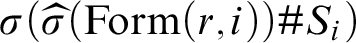 $\sigma (\widehat {\sigma }( \text {Form}(r,i))\# S_i)$
is derivable from the active components of the premises in
$\sigma (\widehat {\sigma }( \text {Form}(r,i))\# S_i)$
is derivable from the active components of the premises in
 $\sigma (\mathcal {H})$
in
$\sigma (\mathcal {H})$
in
 $\mathbf {FL_{e\ast }}$
. We illustrate the case
$\mathbf {FL_{e\ast }}$
. We illustrate the case
 $i\in I$
. The sequent
$i\in I$
. The sequent
 $\sigma (\widehat {\sigma }(\text {Form}(r,i))\# S_i)$
is
$\sigma (\widehat {\sigma }(\text {Form}(r,i))\# S_i)$
is
 $$ \begin{align} \widehat{\sigma}(\text{Form}(r,i)), \sigma({{\mathcal{V}}}_{i}),\sigma(\Gamma_{i1}),\ldots,\sigma(\Gamma_{ir_i}),\sigma(\Sigma_i)\Rightarrow\sigma(\Pi_i). \end{align} $$
From Definition 19 we have that
 $\widehat {\sigma }(\text {Form}(r,i))$
has the following form:
$\widehat {\sigma }(\text {Form}(r,i))$
has the following form:
 $$ \begin{align*} \left({\odot}\sigma({{\mathcal{V}}}_{i})\cdot{\odot}\left\{\sigma(\Gamma_{ij})\land\left(\lnot\bigvee_{l\in M_{ij}}{\odot}\sigma(\vec{{\mathcal{T}}}_{ijl})\right) \mid j\leq r_i\right\} \rightarrow\bigvee_{j\in J_i}{\odot}\sigma({{\mathcal{S}}}_{ij})\right)_{\land 1}. \end{align*} $$
Applying the logical rules backwards to suitably decompose the formula
 $\widehat {\sigma }(\text {Form}(r,i))$
, one obtains a proof of (2) from the active components of
$\widehat {\sigma }(\text {Form}(r,i))$
, one obtains a proof of (2) from the active components of
 $(r)$
. ⊣
$(r)$
. ⊣
Remark 22. An alternative way of obtaining a disjunction formula is by reversing the algorithm in [Reference Ciabattoni, Galatos and Terui12]. The resulting formula would be different, although equivalent, to the one we compute. For example, in absence of weakening, for the (com) rule we would get the formula
 ${(}\widehat {\Gamma }_{2}\rightarrow \widehat {\Gamma }_{1}{)}_{\land 1}\lor (\widehat {\Gamma }_{1}\rightarrow \widehat {\Gamma }_{2}{)}_{\land 1}$
which is slightly simpler than
${(}\widehat {\Gamma }_{2}\rightarrow \widehat {\Gamma }_{1}{)}_{\land 1}\lor (\widehat {\Gamma }_{1}\rightarrow \widehat {\Gamma }_{2}{)}_{\land 1}$
which is slightly simpler than
 $\text {Form}(com)$
in Example 20. The reason for not taking the reversing approach is that the method given here works uniformly for substructural and modal logics, and it does not require any familiarity with the algorithm in [Reference Ciabattoni, Galatos and Terui12].
$\text {Form}(com)$
in Example 20. The reason for not taking the reversing approach is that the method given here works uniformly for substructural and modal logics, and it does not require any familiarity with the algorithm in [Reference Ciabattoni, Galatos and Terui12].
5.3. Multiset-axiomatisations/analyticity for substructural logics
Theorem 23. Let
 $\mathcal {A}$
be an amenable set. Then
$\mathcal {A}$
be an amenable set. Then
 $:$
$:$
-
1. There is a set
$\mathcal {A}'$
computable from
$\mathcal {A}$
such that
$\mathrm {Thm}(\mathbf {FL_{e\ast }}+\mathcal {A}')=\mathrm {Thm}(\mathbf {FL_{e\ast }}+A)$
and
$\mathbf {FL_{e\ast }}+\mathcal {A}'$
is a multiset-analytic sequent calculus. -
2.
$\mathrm {Thm}(\mathbf {FL_{e\ast }}+\mathcal {A})$
is multiset-axiomatisable over
$\mathrm {Thm}(\mathbf {FL_{e\ast }})$
.


Proof. By Theorem 16, we can compute from
 $\mathcal {A}$
a set
$\mathcal {A}$
a set
 $\mathcal {R}_A$
of hypersequent rules such that
$\mathcal {R}_A$
of hypersequent rules such that
 $\mathrm {Thm}(\mathbf {FL_{e\ast }}+\mathcal {A})=\mathrm {Thm}(\mathbf {H}\mathbf {FL_{e\ast }}+\mathcal {R}_A)$
and
$\mathrm {Thm}(\mathbf {FL_{e\ast }}+\mathcal {A})=\mathrm {Thm}(\mathbf {H}\mathbf {FL_{e\ast }}+\mathcal {R}_A)$
and
 $\mathbf {H}\mathbf {FL_{e\ast }}+\mathcal {R}_A$
is analytic. By Definition 19 and Theorem 21, we can compute from the set
$\mathbf {H}\mathbf {FL_{e\ast }}+\mathcal {R}_A$
is analytic. By Definition 19 and Theorem 21, we can compute from the set
 $\mathcal {R}_A$
of rules a set
$\mathcal {R}_A$
of rules a set
 $\mathcal {A}'$
of disjunction forms. Then from Theorem 13 we have that
$\mathcal {A}'$
of disjunction forms. Then from Theorem 13 we have that
 $\mathbf {FL_{e\ast }}+\mathcal {A}'$
is a multiset-analytic sequent calculus, and that
$\mathbf {FL_{e\ast }}+\mathcal {A}'$
is a multiset-analytic sequent calculus, and that
 $\mathrm {Thm}(\mathbf {FL_{e\ast }}+\mathcal {A}')$
is a multiset-axiomatisation over
$\mathrm {Thm}(\mathbf {FL_{e\ast }}+\mathcal {A}')$
is a multiset-axiomatisation over
 $\mathrm {Thm}(\mathbf {FL_{e\ast }})$
w.r.t.
$\mathrm {Thm}(\mathbf {FL_{e\ast }})$
w.r.t.
 $\mathcal {A}'$
. To conclude the proof, it suffices to observe that
$\mathcal {A}'$
. To conclude the proof, it suffices to observe that
 $\mathrm {Thm}(\mathbf {FL_{e\ast }}+\mathcal {A}')=\mathrm {Thm}(\mathbf {H}\mathbf {FL_{e\ast }}+\mathcal {R}_A)=\mathrm {Thm}(\mathbf {FL_{e\ast }}+\mathcal {A})$
.
$\mathrm {Thm}(\mathbf {FL_{e\ast }}+\mathcal {A}')=\mathrm {Thm}(\mathbf {H}\mathbf {FL_{e\ast }}+\mathcal {R}_A)=\mathrm {Thm}(\mathbf {FL_{e\ast }}+\mathcal {A})$
.
6. Stronger forms of boundedness
In the last section we identified a large class of substructural logics that are multiset-axiomatisable. We now consider sufficient conditions for strengthening this result to set- and formula-axiomatisable, and study its consequences. We also study the properties of variable-axiomatisations, which appeared as the ‘simple substitution property’ in the literature.
The stronger forms of axiomatisable rely on the presence of certain structural rules, notably contraction. Formula-axiomatisations (resp. set-axiomatisations) lead to a PTIME (resp. EXPTIME) embedding. An EXPSPACE upper bound then follows for every amenable intermediate logic. It turns out that contraction and mingle suffice for set-axiomatisable. We then obtain a 2EXPTIME upper bound for amenable extensions of
 $\mathbf {FL}_{\mathbf {ecm}\ast }$
. To the best of our knowledge, a bound applying to all these extensions is new. Finally we discuss how variable-axiomatisations can be exploited to obtain interpolation.
$\mathbf {FL}_{\mathbf {ecm}\ast }$
. To the best of our knowledge, a bound applying to all these extensions is new. Finally we discuss how variable-axiomatisations can be exploited to obtain interpolation.
6.1. Set-axiomatisations
Multiset-axiomatisations imply set-axiomatisations whenever the structural rules of contraction and mingle (or weakening) are present.
Lemma 24. Let
 $\mathbf {FL}_{\mathbf {ecm}\ast }+\mathcal {A}$
be multiset-axiomatisable over
$\mathbf {FL}_{\mathbf {ecm}\ast }+\mathcal {A}$
be multiset-axiomatisable over
 $\mathbf {FL_{ecm\ast }}$
. Then
$\mathbf {FL_{ecm\ast }}$
. Then
 $\mathbf {FL_{ecm\ast }}+\mathcal {A}$
is a set-axiomatisable over
$\mathbf {FL_{ecm\ast }}+\mathcal {A}$
is a set-axiomatisable over
 $\mathbf {FL_{ecm\ast }}$
.
$\mathbf {FL_{ecm\ast }}$
.
Proof.
 $\mathbf {FL}_{\mathbf {ecm}\ast }$
establishes
$\mathbf {FL}_{\mathbf {ecm}\ast }$
establishes
 $A\leftrightarrow A\cdot A$
, and hence also its contextualized version
$A\leftrightarrow A\cdot A$
, and hence also its contextualized version
 $B(A)\leftrightarrow B(A\cdot A)$
. From this it follows that for any sets of axioms
$B(A)\leftrightarrow B(A\cdot A)$
. From this it follows that for any sets of axioms
 $\mathcal {A}$
and formula F, the sets
$\mathcal {A}$
and formula F, the sets
 $\mathcal {A}[\psi _{ms}(F)]$
and
$\mathcal {A}[\psi _{ms}(F)]$
and
 $\mathcal {A}[\psi _{s}(F)]$
are equivalent over
$\mathcal {A}[\psi _{s}(F)]$
are equivalent over
 $\mathbf {FL}_{\mathbf {ecm}\ast }$
. ⊣
$\mathbf {FL}_{\mathbf {ecm}\ast }$
. ⊣
Corollary 25. Every amenable extension
 $\mathbf {FL}_{\mathbf {ecm}\ast }+\mathcal {A}$
is set-axiomatisable over
$\mathbf {FL}_{\mathbf {ecm}\ast }+\mathcal {A}$
is set-axiomatisable over
 $\mathbf {FL}_{\mathbf {ecm}\ast }$
.
$\mathbf {FL}_{\mathbf {ecm}\ast }$
.
An embedding of a logic L into a logic K is a function
 $\rho $
on formulas such that
$\rho $
on formulas such that
 $F\in L\leftrightarrow \rho (F)\in K$
. The embedding is PTIME (EXPTIME) if the function is computable in PTIME (EXPTIME).
$F\in L\leftrightarrow \rho (F)\in K$
. The embedding is PTIME (EXPTIME) if the function is computable in PTIME (EXPTIME).
Lemma 26.
-
1. If
$\mathbf {FL_{ec\ast }}+\mathcal {A}$
is a set-axiomatisable over
$\mathbf {FL_{e\ast }}$
then there is an EXPTIME embedding from
$\mathrm {Thm}(\mathbf {FL_{ec\ast }}+\mathcal {A})$
into
$\mathrm {Thm}(\mathbf {FL_{ec\ast }})$
. -
2. If
$\mathbf {FL_{ec\ast }}+\mathcal {A}$
is a formula-axiomatisable over
$\mathbf {FL_{e\ast }}$
then there is a PTIME embedding from
$\mathrm {Thm}(\mathbf {FL_{ec\ast }}+\mathcal {A})$
into
$\mathrm {Thm}(\mathbf {FL_{ec\ast }})$
.


Proof. 1. By the definition of set-axiomatisable,
 $F\in \mathrm {Thm}(\mathbf {FL_{ec\ast }}+\mathcal {A})$
iff
$F\in \mathrm {Thm}(\mathbf {FL_{ec\ast }}+\mathcal {A})$
iff
 $$ \begin{align} \exists A_{1},\ldots,A_{n}\in \psi_s(\mathcal{A},F)\text{ such that } \vdash_{\mathbf{FL_{ec\ast}}} A_{1},\ldots,A_{n}\Rightarrow F. \end{align} $$
Since
 $\psi _s(\mathcal {A},F)$
is a finite set, we have that (*) is equivalent to the following (contraction is needed in the left-to-right direction of the equivalence since a formula
$\psi _s(\mathcal {A},F)$
is a finite set, we have that (*) is equivalent to the following (contraction is needed in the left-to-right direction of the equivalence since a formula
 $A\in \psi _s(\mathcal {A},F)$
might appear multiple times in the list
$A\in \psi _s(\mathcal {A},F)$
might appear multiple times in the list
 $A_1,\ldots,A_n$
).
$A_1,\ldots,A_n$
).
 $$ \begin{align*} \vdash_{\mathbf{FL_{ec\ast}}}{\odot}\{A\land 1\mid A\in \psi_s(\mathcal{A},F)\}\Rightarrow F. \end{align*} $$
Therefore the following is an embedding of
 $\mathrm {Thm}(\mathbf {FL_{ec\ast }}+\mathcal {A})$
into
$\mathrm {Thm}(\mathbf {FL_{ec\ast }}+\mathcal {A})$
into
 $\mathrm {Thm}(\mathbf {FL_{ec\ast }})$
.
$\mathrm {Thm}(\mathbf {FL_{ec\ast }})$
.
 $$ \begin{align*} F \quad\mapsto\quad {\odot}\{A\land 1\mid A\in \psi_s(\mathcal{A},F)\}\rightarrow F. \end{align*} $$
The time to compute values of this function is polynomial in the size of the set
 $\psi _s(\mathcal {A},F)$
and that is exponential in F.
$\psi _s(\mathcal {A},F)$
and that is exponential in F.
2. Arguing as in 1., we see that the following function is an embedding of
 $\mathrm {Thm}(\mathbf {FL_{ec\ast }}+\mathcal {A})$
into
$\mathrm {Thm}(\mathbf {FL_{ec\ast }}+\mathcal {A})$
into
 $\mathrm {Thm}(\mathbf {FL_{ec\ast }})$
.
$\mathrm {Thm}(\mathbf {FL_{ec\ast }})$
.
 $$ \begin{align*} F \quad\mapsto\quad {\odot}\{A\land 1\mid A\in \psi_f(\mathcal{A},F)\}\rightarrow F. \end{align*} $$
It is computable in PTIME because the size of
 $\psi _f(\mathcal {A},F)$
is polynomial in F. ⊣
$\psi _f(\mathcal {A},F)$
is polynomial in F. ⊣
We obtain the following uniform decidability and complexity upper bound.
Corollary 27. Derivability in amenable extensions of
 $\mathbf {FL}_{\mathbf {ecm}\ast }$
is 2
EXPTIME.
$\mathbf {FL}_{\mathbf {ecm}\ast }$
is 2
EXPTIME.
Proof. By Theorem 23 and Lemmas 24 and 26, derivability for every amenable extension of
 $\mathbf {FL_{ecm}}$
can be reduced to derivability in
$\mathbf {FL_{ecm}}$
can be reduced to derivability in
 $\mathbf {FL_{ecm}}$
, in EXPTIME. By Theorem 29 below we have that
$\mathbf {FL_{ecm}}$
, in EXPTIME. By Theorem 29 below we have that
 $\mathrm {Thm}(\mathbf {FL_{ecm}})$
is itself in EXPTIME. The 2EXPTIME upper bound follows.⊣
$\mathrm {Thm}(\mathbf {FL_{ecm}})$
is itself in EXPTIME. The 2EXPTIME upper bound follows.⊣
Example 28. Our decidability and complexity results apply to a large class of logics including Uninorm Mingle Logic
 $\mathbf {UML}$
[Reference Metcalfe and Montagna34] axiomatized as
$\mathbf {UML}$
[Reference Metcalfe and Montagna34] axiomatized as
 $\mathbf {FL_{ecm}}+ (p\rightarrow q)_{\wedge 1}\lor (q \rightarrow p)_{\wedge 1}$
(see [Reference Marchioni and Montagna33] for a proof of decidability), as well as the substructural logics
$\mathbf {FL_{ecm}}+ (p\rightarrow q)_{\wedge 1}\lor (q \rightarrow p)_{\wedge 1}$
(see [Reference Marchioni and Montagna33] for a proof of decidability), as well as the substructural logics
 $\mathbf {FL_{ecm}}+ ((p \cdot \neg p) \to p)_{\wedge 1}$
, and
$\mathbf {FL_{ecm}}+ ((p \cdot \neg p) \to p)_{\wedge 1}$
, and
 $\mathbf {FL_{ecm}}+(Bwk)$
(
$\mathbf {FL_{ecm}}+(Bwk)$
(
 $k\geq 2$
). Here
$k\geq 2$
). Here
 $(Bwk)$
is the well-known formula
$(Bwk)$
is the well-known formula
 $\lor _{i=0}^{k} (p_{i}\rightarrow \lor _{j\neq i} {p_{j}})_{\wedge 1}$
whose addition to intuitionistic logic yields the logic of bounded width intuitionistic Kripke models. ⊣
$\lor _{i=0}^{k} (p_{i}\rightarrow \lor _{j\neq i} {p_{j}})_{\wedge 1}$
whose addition to intuitionistic logic yields the logic of bounded width intuitionistic Kripke models. ⊣
In terms of the algebraic semantics [Reference Galatos, Jipsen, Kowalski and Ono18], the corollary above applies to the equational theory of the corresponding classes of residuated lattices.
A 2EXPTIME upper bound for
 ${\mathbf {FL_{ecm}}}$
already appears in [Reference St John44]. The following improves on this bound. A PSPACE lower bound for this logic was given in [Reference Horcík and Terui21].
${\mathbf {FL_{ecm}}}$
already appears in [Reference St John44]. The following improves on this bound. A PSPACE lower bound for this logic was given in [Reference Horcík and Terui21].
Theorem 29. Derivability in
 ${\mathbf {FL_{ecm}}}$
is EXPTIME.
${\mathbf {FL_{ecm}}}$
is EXPTIME.
Proof. Since
 $\vdash _{{\mathbf {FL_{ecm}}}}^{cf} \Gamma \Rightarrow A$
iff
$\vdash _{{\mathbf {FL_{ecm}}}}^{cf} \Gamma \Rightarrow A$
iff
 $\vdash _{{\mathbf {FL_{ecm}}}}^{cf} \Rightarrow {\odot }\Gamma \rightarrow A$
, it suffices to decide derivability of a formula. Let
$\vdash _{{\mathbf {FL_{ecm}}}}^{cf} \Rightarrow {\odot }\Gamma \rightarrow A$
, it suffices to decide derivability of a formula. Let
 ${\mathbf {FL_{ecm}^s}}$
be the calculus whose rule figures are the same as those of
${\mathbf {FL_{ecm}^s}}$
be the calculus whose rule figures are the same as those of
 ${\mathbf {FL_{ecm}}}$
, but whose sequents have the form
${\mathbf {FL_{ecm}}}$
, but whose sequents have the form
 $X\Rightarrow A$
where X is a set of formulas (instead of a multiset as in
$X\Rightarrow A$
where X is a set of formulas (instead of a multiset as in
 ${\mathbf {FL_{ecm}}}$
). Since
${\mathbf {FL_{ecm}}}$
). Since
 $\vdash _{{\mathbf {FL_{ecm}}}}^{cf} A\leftrightarrow A\cdot A$
, the claim below follows from a standard induction on the height of the derivation.
$\vdash _{{\mathbf {FL_{ecm}}}}^{cf} A\leftrightarrow A\cdot A$
, the claim below follows from a standard induction on the height of the derivation.
 $$ \begin{align*} \text{For every formula}~A\!\!:\ \vdash_{{\mathbf{FL_{ecm}}}}^{cf} \Rightarrow A\ \text{iff}\ \vdash_{{\mathbf{FL_{ecm}^s}}}^{cf}\Rightarrow A. \end{align*} $$
It suffices therefore to search for a proof of
 $\Rightarrow A$
in
$\Rightarrow A$
in
 ${\mathbf {FL_{ecm}^s}}$
. In a cut-free derivation in
${\mathbf {FL_{ecm}^s}}$
. In a cut-free derivation in
 ${\mathbf {FL_{ecm}^s}}$
of
${\mathbf {FL_{ecm}^s}}$
of
 $\Rightarrow A$
, each antecedent is a subset of
$\Rightarrow A$
, each antecedent is a subset of
 $\mathrm {subf}(A)$
. Since
$\mathrm {subf}(A)$
. Since
 $|\mathrm {subf}(A)|\leq |A|$
, there are at most
$|\mathrm {subf}(A)|\leq |A|$
, there are at most
 $2^{|A|}$
such subsets, and at most
$2^{|A|}$
such subsets, and at most
 $|A|$
possibilities for the succedent. There are thus at most
$|A|$
possibilities for the succedent. There are thus at most
 $K:= 2^{|A|}\cdot |A|$
sequents that can occur in a cut-free proof of
$K:= 2^{|A|}\cdot |A|$
sequents that can occur in a cut-free proof of
 $\Rightarrow A$
. Using forward proof search, we can decide in exponential timeFootnote
3
if
$\Rightarrow A$
. Using forward proof search, we can decide in exponential timeFootnote
3
if
 $\Rightarrow A$
is derivable as follows.
$\Rightarrow A$
is derivable as follows.
First, write down on a tape of the Turing Machine, each of the K sequents that can occur in the proof (this takes time polynomial in K). Mark each initial sequent in this list as proved. Now consider the following algorithm:
-
1. For each triple of sequents
$(S_{1},S_{2},S_{3})$
such that
$S_{1}$
and
$S_{2}$
are marked proved and
$S_{3}$
is unmarked, if there is a binary rule instance in
${\mathbf {FL_{ecm}^s}}$
with premises
$S_{1}$
and
$S_{2}$
and conclusion
$S_{3}$
, then mark
$S_{3}$
as newly proved. Proceed similarly with the unary rules of
${\mathbf {FL_{ecm}^s}}$
using a tuple. -
2. If none of the sequents is marked newly proved after Step 1 then terminate. Otherwise, replace every newly proved mark with proved, and go to Step 1.


It is easily verified that
 $\Rightarrow A$
is derivable iff
$\Rightarrow A$
is derivable iff
 $\Rightarrow A$
is marked proved at termination. Step 1 takes time polynomial in K for each triple, and there are at most
$\Rightarrow A$
is marked proved at termination. Step 1 takes time polynomial in K for each triple, and there are at most
 $K^{3}$
different triples (
$K^{3}$
different triples (
 $K^{2}$
different tuples). At each iteration, by Step 2, the algorithm terminates unless the number of sequents marked proved increases. Hence the algorithm must terminate after at most K iterations. It follows that the algorithm has a runtime that is polynomial in K, and thus exponential in
$K^{2}$
different tuples). At each iteration, by Step 2, the algorithm terminates unless the number of sequents marked proved increases. Hence the algorithm must terminate after at most K iterations. It follows that the algorithm has a runtime that is polynomial in K, and thus exponential in
 $|A|$
.
$|A|$
.
6.2. Formula and variable boundedness
The previous subsection made use of contraction and mingle to obtain set-axiomatisations. Replacing mingle with weakening, and hence considering the
 $\mathbf {LJ}$
calculus for intuitionistic logic, opens the door to even sharper results. Here we present two sufficient conditions for a multiset-axiomatisation of
$\mathbf {LJ}$
calculus for intuitionistic logic, opens the door to even sharper results. Here we present two sufficient conditions for a multiset-axiomatisation of
 $\mathbf {LJ}$
to imply a formula-axiomatisation. Adding a further condition implies a variable-axiomatisation and regains the sufficient condition for the simple substitution property presented in [Reference Hosoi23]. Recall that
$\mathbf {LJ}$
to imply a formula-axiomatisation. Adding a further condition implies a variable-axiomatisation and regains the sufficient condition for the simple substitution property presented in [Reference Hosoi23]. Recall that
 $A \wedge 1 \leftrightarrow A$
holds in the presence of weakening, and hence all references to the constant
$A \wedge 1 \leftrightarrow A$
holds in the presence of weakening, and hence all references to the constant
 $1$
are omitted in this section.
$1$
are omitted in this section.
Let
 $A(B/p)$
denote the formula obtained from A by substituting every occurrence of the propositional variable p in A with the formula B.
$A(B/p)$
denote the formula obtained from A by substituting every occurrence of the propositional variable p in A with the formula B.
Definition 30 (
$\Omega $
-propagation property)

Formula A has the
 $\Omega $
-propagation property for a set
$\Omega $
-propagation property for a set
 $\Omega $
of binary connectives if for variables
$\Omega $
of binary connectives if for variables
 $p,q,r$
and every
$p,q,r$
and every
 $\diamond \in C$
,
$\diamond \in C$
,
 $$ \begin{align} \vdash_{\mathbf{LJ}} A(q/p),A(r/p)\Rightarrow A(q\diamond r/p). \end{align} $$
Note that this condition is trivial for variables p not occurring in A.
Lemma 31. Let
 $\mathbf {LJ}+ \mathcal {A}$
be a multiset-axiomatisation over
$\mathbf {LJ}+ \mathcal {A}$
be a multiset-axiomatisation over
 $\mathbf {LJ}$
w.r.t.
$\mathbf {LJ}$
w.r.t.
 $\mathcal {A}$
. It is a formula-axiomatisation if every
$\mathcal {A}$
. It is a formula-axiomatisation if every
 $A\in \mathcal {A}$
has the
$A\in \mathcal {A}$
has the
 $\{\land \}$
-propagation property.
$\{\land \}$
-propagation property.
Proof. Suppose that
 $\vdash _{\mathbf {LJ}+\mathcal {A}}F$
. Since
$\vdash _{\mathbf {LJ}+\mathcal {A}}F$
. Since
 $\mathbf {LJ}+ \mathcal {A}$
is a multiset-axiomatisation, there exist
$\mathbf {LJ}+ \mathcal {A}$
is a multiset-axiomatisation, there exist
 $A_{1},\ldots,A_{n}$
such that
$A_{1},\ldots,A_{n}$
such that
 $\vdash _{\mathbf {LJ}} A_1,\ldots,A_n\Rightarrow F$
and each
$\vdash _{\mathbf {LJ}} A_1,\ldots,A_n\Rightarrow F$
and each
 $A_i$
is a multiset-substitution, i.e., a substitution of the propositional variables of some formula in
$A_i$
is a multiset-substitution, i.e., a substitution of the propositional variables of some formula in
 $\mathcal {A}$
by conjunctions of subformulas of F. By repeatedly using the
$\mathcal {A}$
by conjunctions of subformulas of F. By repeatedly using the
 $\{\land \}$
-propagation property, some sequent
$\{\land \}$
-propagation property, some sequent
 $\vdash _{\mathbf {LJ}} A_1',\ldots,A_m'\Rightarrow F$
is derivable such that each
$\vdash _{\mathbf {LJ}} A_1',\ldots,A_m'\Rightarrow F$
is derivable such that each
 $A_{i}'$
is a substitution of the propositional variables of some formula in
$A_{i}'$
is a substitution of the propositional variables of some formula in
 $\mathcal {A}$
by subformulas of F, i.e., a formula-substitution.⊣
$\mathcal {A}$
by subformulas of F, i.e., a formula-substitution.⊣
Determining if an axiom has the
 $\{\land \}$
-propagation property can be tedious, e.g., try checking this property for the
$\{\land \}$
-propagation property can be tedious, e.g., try checking this property for the
 $Bc_k$
axiom (Kripke models with k worlds)
$Bc_k$
axiom (Kripke models with k worlds)
 $p_0\lor (p_0{\rightarrow } p_1)\lor \cdots \lor (p_0\land \cdots \land p_{k-1}{\rightarrow } p_k)$
.
$p_0\lor (p_0{\rightarrow } p_1)\lor \cdots \lor (p_0\land \cdots \land p_{k-1}{\rightarrow } p_k)$
.
We now introduce an inductive criterion to simplify this check.
In the following, let
 $p\in \mathbf {Var}$
be an arbitrary propositional variable, and let
$p\in \mathbf {Var}$
be an arbitrary propositional variable, and let
 $A(B)$
abbreviate
$A(B)$
abbreviate
 $A(B/p)$
. Let
$A(B/p)$
. Let
 $U_p$
denote the set of formulas that possess the
$U_p$
denote the set of formulas that possess the
 $\{\land \}$
-propagation property with respect to the variable p:
$\{\land \}$
-propagation property with respect to the variable p:
 $$ \begin{align*} U_p = \{A\mid \forall q,r\in \mathbf{Var}.\vdash_{\mathbf{LJ}} A(q),A(r)\Rightarrow A(q\land r)\}. \end{align*} $$
The following is immediate.
Lemma 32. If
 $A\in U_p$
for every variable p occurring in A, then A has the
$A\in U_p$
for every variable p occurring in A, then A has the
 $\{\land \}$
-propagation property.
$\{\land \}$
-propagation property.
Recall that an occurrence of a propositional variable p is negative (positive) in a formula A if it occurs on the left hand side of an odd (resp. even) number of implications. Define the following sets of formulas:
 $$ \begin{align*} U_p^\ast =& \{A\mid\forall q,r\in \mathbf{Var}.\vdash_{\mathbf{LJ}} A(q)\Rightarrow A(q\land r)\}; \\ D_p =& \{A\mid\forall q,r\in \mathbf{Var}.\vdash_{\mathbf{LJ}} A(q\land r)\Rightarrow A(q) \,\&\, \vdash_{\mathbf{LJ}}A(q\land r)\Rightarrow A(r)\};\\ N_p =& \{A\mid\ p \text{occurs only negatively in}~A\}. \end{align*} $$
As a mnemonic, U stands for ‘upwards propagation’ (going from simple instances up to conjunctive instances),
 $U^\ast $
for ‘strong upwards propagation’, D stands for ‘downwards propagation’ (going from conjunctive instances down to simple instances), and of course N stands for negative. For sets
$U^\ast $
for ‘strong upwards propagation’, D stands for ‘downwards propagation’ (going from conjunctive instances down to simple instances), and of course N stands for negative. For sets
 $M,N$
of formulas and a binary connective
$M,N$
of formulas and a binary connective
 $\diamond $
, define
$\diamond $
, define
 $M\diamond N$
to be the set
$M\diamond N$
to be the set
 $\{ A\diamond B\mid A\in M,B\in N\}$
.
$\{ A\diamond B\mid A\in M,B\in N\}$
.
Lemma 33. The following holds.
-
1
$p\in U_p;$
-
2 If p does not occur in
$ A$
, then
$ A\in U^\ast _p\cap U_p\cap D_p;$
-
3
$N_p\subseteq U^\ast _p;$
-
4
$D_p{\rightarrow } U_p\subseteq U_p;$
-
5
$U_p^\ast \lor U_p\subseteq U_p$
.


Proof. (1) Since
 $\vdash _{\mathbf {LJ}} q,r\Rightarrow q\land r$
. (2) holds trivially. (3) Let
$\vdash _{\mathbf {LJ}} q,r\Rightarrow q\land r$
. (2) holds trivially. (3) Let
 $A\in N_p$
, and let
$A\in N_p$
, and let
 $\delta $
be the standard proof of
$\delta $
be the standard proof of
 $A(q)\Rightarrow A(q)$
. Start constructing a proof
$A(q)\Rightarrow A(q)$
. Start constructing a proof
 $\delta '$
of
$\delta '$
of
 $A(q)\Rightarrow A(q\land r)$
bottom up by imitating the proof steps in
$A(q)\Rightarrow A(q\land r)$
bottom up by imitating the proof steps in
 $\delta $
. Whenever the formula
$\delta $
. Whenever the formula
 $q\land r$
appears isolated in
$q\land r$
appears isolated in
 $\delta '$
, then this is on the left hand side of a sequent because
$\delta '$
, then this is on the left hand side of a sequent because
 $A\in N_p$
. We can thus apply a cut with
$A\in N_p$
. We can thus apply a cut with
 $q\land r\Rightarrow q$
to (again, reading the proof bottom up) replace
$q\land r\Rightarrow q$
to (again, reading the proof bottom up) replace
 $q\land r$
with q. Then copy the remaining steps of
$q\land r$
with q. Then copy the remaining steps of
 $\delta $
. (4) Let
$\delta $
. (4) Let
 $A\in D_p$
and
$A\in D_p$
and
 $ B\in U_p$
, and consider the following derivation showing that
$ B\in U_p$
, and consider the following derivation showing that
 $ A{\rightarrow } B\in U_p$
:
$ A{\rightarrow } B\in U_p$
:

(5) Let
 $A\in U_p^\ast $
and
$A\in U_p^\ast $
and
 $B\in U_p$
. Start constructing a proof of
$B\in U_p$
. Start constructing a proof of
 $(A\lor B)(q),(A\lor B)(r)\Rightarrow (A\lor B)(q\land r)$
by applying the rule
$(A\lor B)(q),(A\lor B)(r)\Rightarrow (A\lor B)(q\land r)$
by applying the rule
 $(\lor _L)$
twice. We then have to check provability of the following four sequents:
$(\lor _L)$
twice. We then have to check provability of the following four sequents:
-
(i)
$A(q),A(r)\Rightarrow (A\lor B)(q\land r);$
-
(ii)
$A(q),B(r)\Rightarrow (A\lor B)(q\land r);$
-
(iii)
$B(q),A(r)\Rightarrow (A\lor B)(q\land r);$
-
(iv)
$B(q),B(r)\Rightarrow (A\lor B)(q\land r).$


Now (i)–(iii) are provable since
 $A\in U_p^{\ast }$
. Also (iv) is provable since
$A\in U_p^{\ast }$
. Also (iv) is provable since
 $B\in U_p$
. ⊣
$B\in U_p$
. ⊣
Together, Lemmas 32 and 33 provide a convenient sufficient condition for the
 $\{\land \}$
-propagation property. Here are two examples.
$\{\land \}$
-propagation property. Here are two examples.
Example 34. The
 $\mathbf {Bck}$
axiom
$\mathbf {Bck}$
axiom
 $p_0\lor (p_0{\rightarrow } p_1)\lor \cdots \lor (p_0\land \cdots \land p_{k-1}{\rightarrow } p_k)$
enjoys the
$p_0\lor (p_0{\rightarrow } p_1)\lor \cdots \lor (p_0\land \cdots \land p_{k-1}{\rightarrow } p_k)$
enjoys the
 $\{\land \}$
-propagation property. Indeed by Lemma 33(1)
$\{\land \}$
-propagation property. Indeed by Lemma 33(1)
 $p_{0}$
is in
$p_{0}$
is in
 $U_{p_{0}}$
; by Lemma 33(3) the remaining disjuncts are in
$U_{p_{0}}$
; by Lemma 33(3) the remaining disjuncts are in
 $U^{\ast }_{p_{0}}$
and hence by Lemma 33(5) the axiom is in
$U^{\ast }_{p_{0}}$
and hence by Lemma 33(5) the axiom is in
 $U_{p_{0}}$
. Next observe that by Lemma 33(1,2,4)
$U_{p_{0}}$
. Next observe that by Lemma 33(1,2,4)
 $p_{0}\rightarrow p_{1}$
is in
$p_{0}\rightarrow p_{1}$
is in
 $U_{p_{1}}$
; by Lemma 33(2,3) the remaining disjuncts are in
$U_{p_{1}}$
; by Lemma 33(2,3) the remaining disjuncts are in
 $U^{\ast }_{p_{0}}$
and hence by Lemma 33(5) the axiom is in
$U^{\ast }_{p_{0}}$
and hence by Lemma 33(5) the axiom is in
 $U_{p_{1}}$
. Continuing in this way we can argue that the axiom is in
$U_{p_{1}}$
. Continuing in this way we can argue that the axiom is in
 $U_{p_{i}}$
for all
$U_{p_{i}}$
for all
 $i\leq k$
and hence enjoys the
$i\leq k$
and hence enjoys the
 $\{\land \}$
-propagation property. ⊣
$\{\land \}$
-propagation property. ⊣
Example 35. Consider the linearity axiom
 $ A=(p{\rightarrow } q)\lor (q{\rightarrow } p)$
. To show that
$ A=(p{\rightarrow } q)\lor (q{\rightarrow } p)$
. To show that
 $ A\in U_p$
, we observe that
$ A\in U_p$
, we observe that
 $(p{\rightarrow } q)\in U^\ast _p$
by Lemma 33(3) and
$(p{\rightarrow } q)\in U^\ast _p$
by Lemma 33(3) and
 $(q{\rightarrow } p)\in U_p$
by Lemmas 33(1,2,4). So
$(q{\rightarrow } p)\in U_p$
by Lemmas 33(1,2,4). So
 $A\in U_p$
by Lemma 33(5). By a symmetric argument,
$A\in U_p$
by Lemma 33(5). By a symmetric argument,
 $A\in U_q$
. So by Lemma 32,
$A\in U_q$
. So by Lemma 32,
 $(p{\rightarrow } q)\lor (q{\rightarrow } p)$
has the
$(p{\rightarrow } q)\lor (q{\rightarrow } p)$
has the
 $\{\land \}$
-propagation property and by Lemma 31 we obtain that the standard axiomatisation for Gödel logic
$\{\land \}$
-propagation property and by Lemma 31 we obtain that the standard axiomatisation for Gödel logic
 $\mathbf {LJ}+(p{\rightarrow } q)\lor (q{\rightarrow } p)$
is a formula-axiomatisation. ⊣
$\mathbf {LJ}+(p{\rightarrow } q)\lor (q{\rightarrow } p)$
is a formula-axiomatisation. ⊣
6.3. Variable-axiomatisations
Variable-axiomatisations in intermediate logics were investigated in [Reference Hosoi23, Reference Sasaki40–Reference Sasaki42] as the simple substitution property.
It is important to note that this is a property of a specific axiomatisation rather than a property of the logic, i.e., alternative axiomatisations of the same logic may not have the property. For example, the standard axiomatisation
 $\mathbf {LJ}+(p\rightarrow q)\lor (q\rightarrow p)$
for Gödel logic is not a variable-axiomatisation. The formula
$\mathbf {LJ}+(p\rightarrow q)\lor (q\rightarrow p)$
for Gödel logic is not a variable-axiomatisation. The formula
 $\lnot p\lor \lnot \lnot p$
is a counterexample since it is a theorem of Gödel logic and
$\lnot p\lor \lnot \lnot p$
is a counterexample since it is a theorem of Gödel logic and
 $\mathbf {LJ}$
does not prove
$\mathbf {LJ}$
does not prove
 $(p{\rightarrow } p)\lor (p{\rightarrow } p)\Rightarrow \lnot p\lor \lnot \lnot p$
. As shown in [Reference Sasaki40], a variable-axiomatisation of Gödel logic is
$(p{\rightarrow } p)\lor (p{\rightarrow } p)\Rightarrow \lnot p\lor \lnot \lnot p$
. As shown in [Reference Sasaki40], a variable-axiomatisation of Gödel logic is
 $\mathbf {LJ}+(p{\rightarrow } q)\lor ((p{\rightarrow } q){\rightarrow } p)+(\lnot p\lor \lnot \lnot p).$
A simple sufficient criterion for a variable-axiomatisation is presented in [Reference Hosoi23] using a propagation property. We reformulate that proof in our setting.
Lemma 36. An arbitrary extension
 $\mathbf {LJ}+ \mathcal {A}$
is a variable-axiomatisation w.r.t.
$\mathbf {LJ}+ \mathcal {A}$
is a variable-axiomatisation w.r.t.
 $\mathcal {A}$
if every
$\mathcal {A}$
if every
 $A\in \mathcal {A}$
has the
$A\in \mathcal {A}$
has the
 $\{\land,\lor,\rightarrow \}$
-propagation property.
$\{\land,\lor,\rightarrow \}$
-propagation property.
Proof. If
 $\vdash _{\mathbf {LJ}+\mathcal {A}}(\Rightarrow F)$
for some formula F, then
$\vdash _{\mathbf {LJ}+\mathcal {A}}(\Rightarrow F)$
for some formula F, then
 $\vdash _{\mathbf {LJ}}A_1,\ldots,A_n\Rightarrow F$
for some instances
$\vdash _{\mathbf {LJ}}A_1,\ldots,A_n\Rightarrow F$
for some instances
 $A_i$
of axioms in
$A_i$
of axioms in
 $\mathcal {A}$
. By repeatedly applying the
$\mathcal {A}$
. By repeatedly applying the
 $\{\land,\lor,{\rightarrow }\}$
-propagation property of the axioms, we can replace the list
$\{\land,\lor,{\rightarrow }\}$
-propagation property of the axioms, we can replace the list
 $A_1,\ldots,A_n$
of assumptions by a list
$A_1,\ldots,A_n$
of assumptions by a list
 $A_1',\ldots,A_m'$
of variable instances (i.e., the variables of the axiom substituted by variables). If any variable occurring in some
$A_1',\ldots,A_m'$
of variable instances (i.e., the variables of the axiom substituted by variables). If any variable occurring in some
 $A_{i}'$
does not occur in F, we can uniformly rename such a variable with one that does occur in F. We obtain a proof of
$A_{i}'$
does not occur in F, we can uniformly rename such a variable with one that does occur in F. We obtain a proof of
 $A_1'',\ldots,A_m''\Rightarrow F$
where each
$A_1'',\ldots,A_m''\Rightarrow F$
where each
 $A_i''\in \mathcal {A}[\psi _v(F)]$
. In this way we witness that
$A_i''\in \mathcal {A}[\psi _v(F)]$
. In this way we witness that
 $\mathbf {LJ}+\mathcal {A}$
is a variable-axiomatisation w.r.t.
$\mathbf {LJ}+\mathcal {A}$
is a variable-axiomatisation w.r.t.
 $\mathcal {A}$
. ⊣
$\mathcal {A}$
. ⊣
Observe that Lemma 36 applies to arbitrary extensions of
 $\mathbf {LJ}$
but Lemma 31 requires a multiset-axiomatisation. This is because an arbitrary formula instance
$\mathbf {LJ}$
but Lemma 31 requires a multiset-axiomatisation. This is because an arbitrary formula instance
 $A'$
of
$A'$
of
 $\mathcal {A}$
cannot be transformed to an element of
$\mathcal {A}$
cannot be transformed to an element of
 $\mathcal {A}[\psi _f(F)]$
by variable renaming. In contrast, an arbitrary variable instance
$\mathcal {A}[\psi _f(F)]$
by variable renaming. In contrast, an arbitrary variable instance
 $A'$
of
$A'$
of
 $\mathcal {A}$
is transformable to an element in
$\mathcal {A}$
is transformable to an element in
 $\mathcal {A}[\psi _v(F)]$
via variable renaming. Lemma 36 is used in [Reference Hosoi23] to show that classical logic
$\mathcal {A}[\psi _v(F)]$
via variable renaming. Lemma 36 is used in [Reference Hosoi23] to show that classical logic
 $\mathbf {LJ}+(\lnot p\lor p)$
and
$\mathbf {LJ}+(\lnot p\lor p)$
and
 $\mathbf {LQ}=\mathbf {LJ}+(\lnot p\lor \lnot \lnot p)$
are variable-axiomatisations.
$\mathbf {LQ}=\mathbf {LJ}+(\lnot p\lor \lnot \lnot p)$
are variable-axiomatisations.
A logic L has the Craig interpolation property if
 $A\rightarrow B\in L$
implies the existence of a formula I with
$A\rightarrow B\in L$
implies the existence of a formula I with
 $(A\rightarrow I)\land (I\rightarrow B)\in L$
and
$(A\rightarrow I)\land (I\rightarrow B)\in L$
and
 $\mathbf {Var}(I)\subseteq \mathbf {Var}(A)\cap \mathbf {Var}(B)$
. We reproduce below the elegant argument from [Reference Sasaki40] where the Craig interpolation property for
$\mathbf {Var}(I)\subseteq \mathbf {Var}(A)\cap \mathbf {Var}(B)$
. We reproduce below the elegant argument from [Reference Sasaki40] where the Craig interpolation property for
 $\mathbf {LQ}$
is induced from
$\mathbf {LQ}$
is induced from
 $\mathbf {LJ}$
by using a variable-axiomatisation. An analogous argument applies to classical logic.
$\mathbf {LJ}$
by using a variable-axiomatisation. An analogous argument applies to classical logic.
Theorem 37.
 $\mathbf {LQ}$
has the Craig interpolation property.
$\mathbf {LQ}$
has the Craig interpolation property.
Proof. For a formula X, let
 $A_X$
denote the conjunction of all formulas
$A_X$
denote the conjunction of all formulas
 $\lnot q\lor \lnot \lnot q$
such that
$\lnot q\lor \lnot \lnot q$
such that
 $q\in \mathbf {Var}(X)$
. If
$q\in \mathbf {Var}(X)$
. If
 $\vdash _{\mathbf {LQ}}B{\rightarrow } C$
, then since
$\vdash _{\mathbf {LQ}}B{\rightarrow } C$
, then since
 $\mathbf {LQ}$
is a variable-axiomatisation over
$\mathbf {LQ}$
is a variable-axiomatisation over
 $\mathbf {LJ}$
w.r.t.
$\mathbf {LJ}$
w.r.t.
 $(\lnot p\lor \lnot \lnot p)$
we know
$(\lnot p\lor \lnot \lnot p)$
we know
 $\vdash _{\mathbf {LJ}} A_{B{\rightarrow } C}{\rightarrow }(B{\rightarrow } C)$
. Since
$\vdash _{\mathbf {LJ}} A_{B{\rightarrow } C}{\rightarrow }(B{\rightarrow } C)$
. Since
 $\lnot q\lor \lnot \lnot q$
has only one variable, every conjunct in
$\lnot q\lor \lnot \lnot q$
has only one variable, every conjunct in
 $A_{B}\land A_{C}$
appears in
$A_{B}\land A_{C}$
appears in
 $A_{B{\rightarrow } C}$
and vice versa. Thus
$A_{B{\rightarrow } C}$
and vice versa. Thus
 $\vdash _{\mathbf {LJ}} A_{B{\rightarrow } C}\leftrightarrow A_{B}\land A_C$
, and hence
$\vdash _{\mathbf {LJ}} A_{B{\rightarrow } C}\leftrightarrow A_{B}\land A_C$
, and hence
 $\vdash _{\mathbf {LJ}} (A_B\land A_C){\rightarrow }(B{\rightarrow } C)$
. It follows that
$\vdash _{\mathbf {LJ}} (A_B\land A_C){\rightarrow }(B{\rightarrow } C)$
. It follows that
 $\vdash _{\mathbf {LJ}} (A_B\land B){\rightarrow } (A_C{\rightarrow } C)$
. By the interpolation property of
$\vdash _{\mathbf {LJ}} (A_B\land B){\rightarrow } (A_C{\rightarrow } C)$
. By the interpolation property of
 $\mathbf {LJ}$
, there is a formula I such that
$\mathbf {LJ}$
, there is a formula I such that
 $\mathbf {Var}(I)\subseteq \mathbf {Var}(A)\cap \mathbf {Var}(B)$
and
$\mathbf {Var}(I)\subseteq \mathbf {Var}(A)\cap \mathbf {Var}(B)$
and
 $\vdash _{\mathbf {LJ}} ((A_B\land B){\rightarrow } I) \land (I{\rightarrow }(A_C{\rightarrow } C)$
. Then the latter formula is also provable in
$\vdash _{\mathbf {LJ}} ((A_B\land B){\rightarrow } I) \land (I{\rightarrow }(A_C{\rightarrow } C)$
. Then the latter formula is also provable in
 $\mathbf {LQ}$
. Since
$\mathbf {LQ}$
. Since
 $A_B,A_C\in \mathbf {LQ}$
, by rearranging and some cuts
$A_B,A_C\in \mathbf {LQ}$
, by rearranging and some cuts
 $\vdash _{\mathbf {LQ}} (B{\rightarrow } I) \land (I{\rightarrow } C)$
. Hence I is a Craig interpolant of
$\vdash _{\mathbf {LQ}} (B{\rightarrow } I) \land (I{\rightarrow } C)$
. Hence I is a Craig interpolant of
 $A{\rightarrow } B$
in
$A{\rightarrow } B$
in
 $\mathbf {LQ}$
.⊣
$\mathbf {LQ}$
.⊣
In [Reference Sasaki41] it is shown that classical logic and
 $\mathbf {LQ}$
are the only consistent variable-axiomatisable logics over
$\mathbf {LQ}$
are the only consistent variable-axiomatisable logics over
 $\mathbf {LJ}$
that are axiomatisable by a single-variable formula. The same paper shows that all finite-valued Gödel logics are variable-axiomatisable over
$\mathbf {LJ}$
that are axiomatisable by a single-variable formula. The same paper shows that all finite-valued Gödel logics are variable-axiomatisable over
 $\mathbf {LJ}$
. We remark that these results have been generalised in [Reference Sasaki42] using algebraic methods to establish necessary and sufficient criterion for variable-axiomatisable intermediate logics on a finite slice (see [Reference Hosoi22]).
$\mathbf {LJ}$
. We remark that these results have been generalised in [Reference Sasaki42] using algebraic methods to establish necessary and sufficient criterion for variable-axiomatisable intermediate logics on a finite slice (see [Reference Hosoi22]).
7. Methodology extended to modal logics
In this section we demonstrate how the methodology applies to other non-classical logics, taking here the example of modal logics. In Section 7.1 we establish formula-axiomatisations for the case study of
 $\mathbf {S4.2}$
. Next we apply our methodology to the uniform hypersequent calculi in [Reference Lahav29] for a large class of modal logics extending
$\mathbf {S4.2}$
. Next we apply our methodology to the uniform hypersequent calculi in [Reference Lahav29] for a large class of modal logics extending
 $\mathbf {S4}$
by Lahav’s simple frame properties. Finally, in Section 7.3 we sharpen the technique even further to obtain a new syntactic proof of a well-known result: the sequent calculus for
$\mathbf {S4}$
by Lahav’s simple frame properties. Finally, in Section 7.3 we sharpen the technique even further to obtain a new syntactic proof of a well-known result: the sequent calculus for
 $\mathbf {S5}$
is analytic.
$\mathbf {S5}$
is analytic.
7.1. Formula-axiomatisation of
$\mathbf {S4.2}$

Throughout, a formula is called boxed if it has the form
 $\Box A$
.
$\Box A$
.
The modal logic
 $\mathbf {S4}$
of pre-ordered (reflexive and transitive) Kripke frames is obtained by the addition of the following two rules to the standard multi-conclusion sequent calculus
$\mathbf {S4}$
of pre-ordered (reflexive and transitive) Kripke frames is obtained by the addition of the following two rules to the standard multi-conclusion sequent calculus
 $\mathbf {LK}$
for classical propositional logic.
$\mathbf {LK}$
for classical propositional logic.

The modal logic
 $\mathbf {S4.2}$
extends
$\mathbf {S4.2}$
extends
 $\mathbf {S4}$
by the axiom
$\mathbf {S4}$
by the axiom
 $\Diamond \Box p{\rightarrow }\Box \Diamond p$
. This logic is characterised semantically as the logic of directed pre-ordered Kripke frames. A cut-free hypersequent calculus
$\Diamond \Box p{\rightarrow }\Box \Diamond p$
. This logic is characterised semantically as the logic of directed pre-ordered Kripke frames. A cut-free hypersequent calculus
 $\mathbf {HS4.2}$
for
$\mathbf {HS4.2}$
for
 $\mathbf {S4.2}$
is obtained (see [Reference Kurokawa, Nakano, Satoh and Bekki28]) by lifting
$\mathbf {S4.2}$
is obtained (see [Reference Kurokawa, Nakano, Satoh and Bekki28]) by lifting
 $\mathbf {S4}$
to a hypersequent calculus
$\mathbf {S4}$
to a hypersequent calculus
 $\mathbf {HS4}$
and then adding the modal rule
$\mathbf {HS4}$
and then adding the modal rule

Paralleling the argument in Section 4.2, we now transform cut-free
 $\mathbf {HS4.2}$
-proofs into bounded analytic sequent calculus proofs. First, using the rules
$\mathbf {HS4.2}$
-proofs into bounded analytic sequent calculus proofs. First, using the rules
 $(ec)$
and
$(ec)$
and
 $(w_l)$
it is easy to see that any instance of
$(w_l)$
it is easy to see that any instance of
 $(RMS)$
can be replaced by multiple applications of its single formula variant
$(RMS)$
can be replaced by multiple applications of its single formula variant

As a disjunction form for
 $(RMS_1)$
, we choose the formula
$(RMS_1)$
, we choose the formula
 $\Box \lnot \Box \Box p\lor \Box \lnot \Box \lnot \Box p$
(the formal computation of the modal disjunction form is explained in Section 7.2). This is equivalent to the axiom instance
$\Box \lnot \Box \Box p\lor \Box \lnot \Box \lnot \Box p$
(the formal computation of the modal disjunction form is explained in Section 7.2). This is equivalent to the axiom instance
 $\Diamond \Box (\Box p){\rightarrow }\Box \Diamond (\Box p)$
and hence the provability property is satisfied. The following two derivations show the splitting property for
$\Diamond \Box (\Box p){\rightarrow }\Box \Diamond (\Box p)$
and hence the provability property is satisfied. The following two derivations show the splitting property for
 $\sigma (p)=A$
:
$\sigma (p)=A$
:

We can then eliminate applications of
 $(RMS_1)$
in proofs of
$(RMS_1)$
in proofs of
 ${\Rightarrow } F$
by adding the formula
${\Rightarrow } F$
by adding the formula
 $\Box \lnot \Box \Box A$
or the formula
$\Box \lnot \Box \Box A$
or the formula
 $\Box \lnot \Box \lnot \Box A$
into the corresponding antecedent of the rule conclusion. We then propagate these formulas downwards in each of the two derivations. Crucially, since both formulas are boxed, adding them to the antecedent of applications of
$\Box \lnot \Box \lnot \Box A$
into the corresponding antecedent of the rule conclusion. We then propagate these formulas downwards in each of the two derivations. Crucially, since both formulas are boxed, adding them to the antecedent of applications of
 $(4)$
yields a legal instance of
$(4)$
yields a legal instance of
 $(4)$
.
$(4)$
.
Finally, combine the two derivations by a disjunction introduction to obtain a proof of
 $\Box \lnot \Box \Box A\lor \Box \lnot \Box \lnot \Box A\Rightarrow F$
. As
$\Box \lnot \Box \Box A\lor \Box \lnot \Box \lnot \Box A\Rightarrow F$
. As
 $\Box A$
appeared in the cut-free hypersequent calculus proof, it must be a subformula of F. Eliminate all instances of
$\Box A$
appeared in the cut-free hypersequent calculus proof, it must be a subformula of F. Eliminate all instances of
 $(RMS_1)$
and reduce the resulting
$(RMS_1)$
and reduce the resulting
 $\mathbf {HS4}$
proof into a sequent calculus proof.
$\mathbf {HS4}$
proof into a sequent calculus proof.
Theorem 38. The logic
 $\mathbf {S4.2}$
is formula-axiomatisable over
$\mathbf {S4.2}$
is formula-axiomatisable over
 $\mathbf {S4}$
. In other words, this means
$\mathbf {S4}$
. In other words, this means
 $F \in \mathbf {S4.2}$
iff there are boxed subformulas
$F \in \mathbf {S4.2}$
iff there are boxed subformulas
 $A_1,\ldots,A_n$
of F such that
$A_1,\ldots,A_n$
of F such that
 $\bigwedge _{i=1}^n (\Box \lnot \Box A_i\lor \Box \lnot \Box \lnot A_i){\rightarrow } F\in \mathbf {S4}$
.
$\bigwedge _{i=1}^n (\Box \lnot \Box A_i\lor \Box \lnot \Box \lnot A_i){\rightarrow } F\in \mathbf {S4}$
.
We obtain formula-axiomatisations—as opposed to set-axiomatisations—because we replaced
 $\Box \Gamma $
in
$\Box \Gamma $
in
 $(RMS)$
with
$(RMS)$
with
 $\Box A$
in
$\Box A$
in
 $(RMS_{1})$
.
$(RMS_{1})$
.
7.2. Bounded-analytic sequent calculi for simple frame properties
Bounded-analytic sequent calculi for modal logics—extending the methodology for substructural logics—can be obtained from a uniform presentation of the hypersequent rules. We illustrate using the rules in [Reference Lahav29] for extensions of
 $\mathbf {S4}$
.
$\mathbf {S4}$
.
Let n be a positive natural number and
 $S=\{ (S_{R}^{i},S_{=}^{i}) \}_{i\in I}$
for some finite index set I such that every
$S=\{ (S_{R}^{i},S_{=}^{i}) \}_{i\in I}$
for some finite index set I such that every
 $S_{R}^{i}$
and
$S_{R}^{i}$
and
 $S_{=}^{i}$
is a subset of
$S_{=}^{i}$
is a subset of
 $\{1,\dots,n\}$
and every
$\{1,\dots,n\}$
and every
 $S_{R}^{i} \cup S_{=}^{i}$
is non-empty. This is what is called a “normal description of an n-simple
$S_{R}^{i} \cup S_{=}^{i}$
is non-empty. This is what is called a “normal description of an n-simple
 $\mathcal {L}_{1}$
-formula” [Reference Lahav29, Definition 4]. Any such description defines a first-order formula
$\mathcal {L}_{1}$
-formula” [Reference Lahav29, Definition 4]. Any such description defines a first-order formula
 $$ \begin{align*} \forall w_{1}\ldots\forall w_{n}\exists u\bigvee_{i\in I}\left(\bigwedge_{i\in S_{R}^{i}} w_{i}Ru \land \bigwedge_{i\in S_{=}^{i}} w_{i}=u\right) .\end{align*} $$
This gives rise to the class of Kripke frames satisfying this formula. The modal logic of S is defined as the set of formulas valid on this class of frames. For each such logic, an analytic hypersequent calculus is obtained in [Reference Lahav29] by computing the following hypersequent rule “induced by S for transitive modal logics”

 $\Box \Gamma _{i}$
and
$\Box \Gamma _{i}$
and
 $\boxtimes \Gamma _{i}$
are standard notation for multiset schematic-variables that are instantiable by sets
$\boxtimes \Gamma _{i}$
are standard notation for multiset schematic-variables that are instantiable by sets
 $\{\Box A_{1},\ldots,\Box A_{k}\}$
and
$\{\Box A_{1},\ldots,\Box A_{k}\}$
and
 $\{A_{1},\Box A_{1},\ldots,A_{k},\Box A_{k}\}$
respectively.
$\{A_{1},\Box A_{1},\ldots,A_{k},\Box A_{k}\}$
respectively.
-
– Set
$S_{lin}=\{(S_{R}^{i}, S_{=}^{i})\}_{i\in \{1,2\}}$
with
$S_{R}^{1}=\{1\}$
,
$S_{=}^{1}=\{2\}$
,
$S_{R}^{2}=\{2\}$
, and
$S_{=}^{2}=\{1\}$
. The modal logic of
$S_{lin}$
is the set of modal formulas valid on the class of frames satisfying
$\forall w_{1}w_{2}\exists u. (w_{1}Ru \land w_{2}=u)\lor (w_{2}Ru \land w_{1}=u)$
. This defines the analytic ruleTherefore
$\mathbf {HS4}+r(S_{lin})$
is a cut-free hypersequent calculus for
$S_{lin}$
. -
– For
$S= \{ (\{i,j\},\emptyset ) | 1\leq i<j\leq n\}$
, the corresponding first-order formula is
$\forall w_{1}\ldots \forall w_{n}\exists u\bigvee _{1\leq i<j\leq n}(w_{i}=u\land w_{j}=u)$
(bounded cardinality) and the hypersequent rule is


We shall obtain the following analogue of Theorem 13 for the function
 $\text {Form}^{\Box }$
defined below that maps an analytic hypersequent rule to a modal formula.
$\text {Form}^{\Box }$
defined below that maps an analytic hypersequent rule to a modal formula.
Theorem 40. For every normal description S and the analytic hypersequent rules
 $\mathcal {R}$
induced by it, the modal logic
$\mathcal {R}$
induced by it, the modal logic
 $\mathrm {Thm}(\mathbf {HS4}+\mathcal {R})$
is a set-axiomatisation over
$\mathrm {Thm}(\mathbf {HS4}+\mathcal {R})$
is a set-axiomatisation over
 $\mathbf {S4}$
w.r.t.
$\mathbf {S4}$
w.r.t.
 $\{{{\text {Form}^{\Box }(R)}} | R\in \mathcal {R}\}$
.
$\{{{\text {Form}^{\Box }(R)}} | R\in \mathcal {R}\}$
.
Proof. Let the normal description
 $S=\{ (S_{R}^{i},S_{=}^{i}) \}_{i\in I}$
be given.
$S=\{ (S_{R}^{i},S_{=}^{i}) \}_{i\in I}$
be given.
In order to compute the disjunction form for the hypersequent rule induced by S, we first rewrite the rule as follows:

In the above, we have partitioned
 $I=I_{1}\sqcup I_{2}$
such that
$I=I_{1}\sqcup I_{2}$
such that
 $S_{=}^{i} = \emptyset $
iff
$S_{=}^{i} = \emptyset $
iff
 $i\in I_{2}$
. For the purpose of obtaining an association form as done in Section 5.2 we begin by reading
$i\in I_{2}$
. For the purpose of obtaining an association form as done in Section 5.2 we begin by reading
 $\Box \Gamma _{j}'$
and
$\Box \Gamma _{j}'$
and
 $\boxtimes \Gamma _{j}'$
as the same multiset schematic-variable. Following that algorithm, the distinguished variable occurrences of each active component in the premises are: some
$\boxtimes \Gamma _{j}'$
as the same multiset schematic-variable. Following that algorithm, the distinguished variable occurrences of each active component in the premises are: some
 $\Sigma _{j}$
(
$\Sigma _{j}$
(
 $j\in S_{=}^{i}$
) for
$j\in S_{=}^{i}$
) for
 $i\in I_{1}$
, and some
$i\in I_{1}$
, and some
 $\boxtimes \Gamma _{j}'$
(
$\boxtimes \Gamma _{j}'$
(
 $j\in S_{R}^{i}$
) for
$j\in S_{R}^{i}$
) for
 $i\in I_{2}$
. Associating
$i\in I_{2}$
. Associating
 $\Box \Gamma _{j}'$
and
$\Box \Gamma _{j}'$
and
 $\boxtimes \Gamma _{j}'$
to the same propositional variable, construct
$\boxtimes \Gamma _{j}'$
to the same propositional variable, construct
 $\text {Form}(r(S))$
from the association form (Definition 19). The required formula
$\text {Form}(r(S))$
from the association form (Definition 19). The required formula
 ${{\text {Form}^{\Box }(r(S))}}$
is obtained by amending
${{\text {Form}^{\Box }(r(S))}}$
is obtained by amending
 $\text {Form}(r(S))$
as follows:
$\text {Form}(r(S))$
as follows:
-
(i) Replace every leading disjunct
$B\land 1$
by B (if B is boxed) or
$\Box B$
(otherwise). -
(ii) A
$\Box $
is placed in front of every propositional variable.


Now follow the proof for
 $\text {Form}(r(S))$
(Theorem 21) to prove that
$\text {Form}(r(S))$
(Theorem 21) to prove that
 ${{\text {Form}^{\Box }(r(S))}}$
is a disjunction formula (provability, weakening, and splitting property). Regarding the amendments, observe that these can be emulated by applying the appropriate modal rules: for (i), use (4) to introduce a leading
${{\text {Form}^{\Box }(r(S))}}$
is a disjunction formula (provability, weakening, and splitting property). Regarding the amendments, observe that these can be emulated by applying the appropriate modal rules: for (i), use (4) to introduce a leading
 $\Box $
; for (ii), start with
$\Box $
; for (ii), start with
 $\Box p\Rightarrow \Box p$
rather than
$\Box p\Rightarrow \Box p$
rather than
 $p\Rightarrow p$
. We do have to account for our reading of
$p\Rightarrow p$
. We do have to account for our reading of
 $\Box \Gamma _{j}'$
and
$\Box \Gamma _{j}'$
and
 $\boxtimes \Gamma _{j}'$
as the same variable despite these multiset schematic-variables having different instantiations (the former permits instantiation only by
$\boxtimes \Gamma _{j}'$
as the same variable despite these multiset schematic-variables having different instantiations (the former permits instantiation only by
 $\{\Box A_{1},\ldots,\Box A_{k}\}$
and the latter only by
$\{\Box A_{1},\ldots,\Box A_{k}\}$
and the latter only by
 $\{A_{1},\Box A_{1},\ldots,A_{k},\Box A_{k}\}$
). It turns out that this is not problematic because every instantiation of “strong box variable
$\{A_{1},\Box A_{1},\ldots,A_{k},\Box A_{k}\}$
). It turns out that this is not problematic because every instantiation of “strong box variable
 $\Rightarrow $
its box variable” and “box variable
$\Rightarrow $
its box variable” and “box variable
 $\Rightarrow $
its strong box variable” is derivable in
$\Rightarrow $
its strong box variable” is derivable in
 $\mathbf {S4}$
.
$\mathbf {S4}$
.

To obtain a multiset-axiomatisation we follow the proof of Theorem 13. The only thing to check is that each disjunct in the disjunction form can be permuted downwards, i.e., adding this formula to the antecedents of the premise(s) and conclusion of a rule instance should not invalidate the rule instance. This holds for the instances of the
 $(4)$
rule because this formula is boxed due to (i), and it is immediate for the other rules. Finally, a set-axiomatisation follows from the presence of contraction and weakening, refer to Lemma 24. ⊣
$(4)$
rule because this formula is boxed due to (i), and it is immediate for the other rules. Finally, a set-axiomatisation follows from the presence of contraction and weakening, refer to Lemma 24. ⊣
The above proof relies on the presence of the
 $(T)$
and
$(T)$
and
 $(4)$
rules. In particular, if the
$(4)$
rules. In particular, if the
 $(4)$
rule was replaced by the standard modal rule for
$(4)$
rule was replaced by the standard modal rule for
 $\mathbf {K}$
, then the addition of a boxed formula to the premise and conclusion of the latter would invalidate the rule instance. This is why the theorem is framed with respect to
$\mathbf {K}$
, then the addition of a boxed formula to the premise and conclusion of the latter would invalidate the rule instance. This is why the theorem is framed with respect to
 $\mathbf {S4}$
.
$\mathbf {S4}$
.
Example 41. Consider
 $r(S_{lin})$
in Example 39. Read
$r(S_{lin})$
in Example 39. Read
 $\Box \Gamma _{1}'$
and
$\Box \Gamma _{1}'$
and
 $\boxtimes \Gamma _{1}'$
as the same variable, and read
$\boxtimes \Gamma _{1}'$
as the same variable, and read
 $\Box \Gamma _{2}'$
and
$\Box \Gamma _{2}'$
and
 $\boxtimes \Gamma _{2}'$
as the same variable to obtain the association form. Associating
$\boxtimes \Gamma _{2}'$
as the same variable to obtain the association form. Associating
 $\Box \Gamma _{1}'$
and
$\Box \Gamma _{1}'$
and
 $\boxtimes \Gamma _{1}'$
with the propositional variable p, and
$\boxtimes \Gamma _{1}'$
with the propositional variable p, and
 $\Box \Gamma _{2}'$
and
$\Box \Gamma _{2}'$
and
 $\boxtimes \Gamma _{2}'$
with the propositional variable q, we obtain
$\boxtimes \Gamma _{2}'$
with the propositional variable q, we obtain
 $$ \begin{align*} \text{Form}(r(S_{lin})):= ((p\rightarrow q){\land 1})\lor ((q\rightarrow p){\land 1}). \end{align*} $$
Applying (i) we get
 $\Box (p\rightarrow q)\lor \Box (q\rightarrow p)$
. After (ii) we obtain
$\Box (p\rightarrow q)\lor \Box (q\rightarrow p)$
. After (ii) we obtain
 $$ \begin{align*} {{\text{Form}^{\Box}(r(S_{lin}))}}:= \Box (\Box p\rightarrow \Box q)\lor \Box (\Box q\rightarrow \Box p). \end{align*} $$
Let us prove that
 $\Box (\Box p\rightarrow \Box q)\lor \Box (\Box q\rightarrow \Box p)$
is a disjunction form of
$\Box (\Box p\rightarrow \Box q)\lor \Box (\Box q\rightarrow \Box p)$
is a disjunction form of
 $r(S_{lin})$
. The following derivation in
$r(S_{lin})$
. The following derivation in
 $\mathbf {HS4}$
witnesses one half of the splitting property (the other derivation is analogous).
$\mathbf {HS4}$
witnesses one half of the splitting property (the other derivation is analogous).

Observe that the instance of the right disjunct of the disjunction formula above is obtained by the substitution
 $q\mapsto \land \Box \Gamma _{2}'$
and
$q\mapsto \land \Box \Gamma _{2}'$
and
 $p\mapsto \land \Box \Gamma _{1}'$
, analogous to the substructural case. The following establishes the provability property.
$p\mapsto \land \Box \Gamma _{1}'$
, analogous to the substructural case. The following establishes the provability property.

7.3. A new syntactic proof of analyticity for
$\mathbf {S5}$

A sequent calculus for
 $\mathbf {S5}$
is obtained by the addition of the rules
$\mathbf {S5}$
is obtained by the addition of the rules
 $(T)$
and
$(T)$
and
 $(5)$
to the sequent calculus
$(5)$
to the sequent calculus
 $\mathbf {LK}$
for classical propositional logic:
$\mathbf {LK}$
for classical propositional logic:

In response to the failure of cut-elimination for this calculus, Takano [Reference Takano45] gave an intricate syntactic proof of analyticity, establishing that only cuts on subformulas are required. Prior to that, only a semantic argument had been shown, see [Reference Fitting17].
A formula-axiomatisation for
 $\mathbf {S5}$
can be established along the lines of Theorem 38. Is it possible to tweak the methodology of this paper to obtain Takano’s (stronger) analyticity result? The answer is affirmative, as shown below.
$\mathbf {S5}$
can be established along the lines of Theorem 38. Is it possible to tweak the methodology of this paper to obtain Takano’s (stronger) analyticity result? The answer is affirmative, as shown below.
Theorem 42. The sequent calculus for
 $\mathbf {S5}$
is analytic.
$\mathbf {S5}$
is analytic.
Proof. Our starting point is a cut-free hypersequent calculus for
 $\mathbf {S5}$
presented in [Reference Kurokawa, Nakano, Satoh and Bekki28]. It extends
$\mathbf {S5}$
presented in [Reference Kurokawa, Nakano, Satoh and Bekki28]. It extends
 $\mathbf {HS4}$
by the rule
$\mathbf {HS4}$
by the rule

This is a special case of Avron’s rule
 $(MS_{Av})$
(cf. Example 2). Cut-free
$(MS_{Av})$
(cf. Example 2). Cut-free
 $\mathbf {HS4}+{(MS)}$
derives exactly the same sequents as the sequent calculus for
$\mathbf {HS4}+{(MS)}$
derives exactly the same sequents as the sequent calculus for
 $\mathbf {S5}$
. Moreover, any instance of the rule
$\mathbf {S5}$
. Moreover, any instance of the rule
 ${(MS)}$
can be simulated using
${(MS)}$
can be simulated using
 $(ec)$
,
$(ec)$
,
 $(w_l)$
, and using multiple instances of its single formula version
$(w_l)$
, and using multiple instances of its single formula version
 ${(MS_1)}$
below:
${(MS_1)}$
below:

Consider a cut-free derivation d in
 $\mathbf {HS4}+{(MS_1)}$
of a sequent S. For simplicity, suppose that d contains a single instance of
$\mathbf {HS4}+{(MS_1)}$
of a sequent S. For simplicity, suppose that d contains a single instance of
 ${(MS_1)}$
(in the general case, bottommost instances of
${(MS_1)}$
(in the general case, bottommost instances of
 ${(MS_1)}$
are eliminated at each step, refer to the proof of Theorem 13). From this instance, we can obtain the following derivations in
${(MS_1)}$
are eliminated at each step, refer to the proof of Theorem 13). From this instance, we can obtain the following derivations in
 $\mathbf {HS4}+{(MS_1)}$
:
$\mathbf {HS4}+{(MS_1)}$
:

Above left (right), the component
 $\Box A\Rightarrow \Box A$
(resp.
$\Box A\Rightarrow \Box A$
(resp.
 $\Box A,\Gamma \Rightarrow \Pi $
) has a
$\Box A,\Gamma \Rightarrow \Pi $
) has a
 $\Box A$
in the succedent (resp. antecedent) that was not present in the original derivation d. Proceed downward from each hypersequent mimicking the rules in d. Although these hypersequents each contain an additional occurrence of
$\Box A$
in the succedent (resp. antecedent) that was not present in the original derivation d. Proceed downward from each hypersequent mimicking the rules in d. Although these hypersequents each contain an additional occurrence of
 $\Box A$
that needs to be propagated downwards, the same rule can be used for this purpose provided it is not
$\Box A$
that needs to be propagated downwards, the same rule can be used for this purpose provided it is not
 $(4)$
. The issue with
$(4)$
. The issue with
 $(4)$
is that it permits only a single formula in the succedent and the additional
$(4)$
is that it permits only a single formula in the succedent and the additional
 $\Box A$
in the succedent would violate this. The solution is to use
$\Box A$
in the succedent would violate this. The solution is to use
 $(5)$
instead. In this way we obtain
$(5)$
instead. In this way we obtain
 ${(MS_1)}$
-free hypersequent derivations (hence in
${(MS_1)}$
-free hypersequent derivations (hence in
 $\mathbf {HS5}$
) of
$\mathbf {HS5}$
) of
 $\Box A\# S$
and
$\Box A\# S$
and
 $S\# \Box A$
(the latter denotes that
$S\# \Box A$
(the latter denotes that
 $\Box A$
is added to the succedent of S). Applying the cut-rule on
$\Box A$
is added to the succedent of S). Applying the cut-rule on
 $\Box A$
on these sequents, we obtain a derivation of S in
$\Box A$
on these sequents, we obtain a derivation of S in
 $\mathbf {HS5}$
. Since
$\mathbf {HS5}$
. Since
 $\Box A$
occurred in the cut-free derivation d, it is a subformula of S. Since every rule in
$\Box A$
occurred in the cut-free derivation d, it is a subformula of S. Since every rule in
 $\mathbf {HS5}$
has one active component, we can extract an analytic derivation of S in the sequent calculus for
$\mathbf {HS5}$
has one active component, we can extract an analytic derivation of S in the sequent calculus for
 $\mathbf {S5}$
.⊣
$\mathbf {S5}$
.⊣
8. Conclusions and open problems
We investigated generalisations of the subformula property that enabled us to retain the simplicity of the sequent calculus for various families of logics, and to establish meta-logical properties. This represents a departure from the typical approach in structural proof theory where the subformula property is treated as the primary goal, even if this means structural enrichment and new proof formalisms; think, e.g., the
 $|$
in the hypersequent calculus, the nesting of structural parentheses in the nested sequent calculus, or the display calculus [Reference Belnap8] where each logical connective corresponds to a structural one. While the difficulties of dealing with an enriched structural language are well known, a formal assessment of this cost has never been investigated. Our transformations suggest a nuanced assessment method by pegging the strength of the subformula property in the hypersequent calculus to restrictions of the axiom instances. We aim to extend these transformations to formalisms beyond the hypersequent calculus such as the nested sequent (preliminary work along this line appears in [Reference Pimentel, Ramanayake, Lellmann, Cerrito and Popescu37]), display calculus, and bunched sequent calculus. This could pave the way for a new classification of logics and formalisms, according to the degree of boundedness of their bounded-analytic sequent calculi.
$|$
in the hypersequent calculus, the nesting of structural parentheses in the nested sequent calculus, or the display calculus [Reference Belnap8] where each logical connective corresponds to a structural one. While the difficulties of dealing with an enriched structural language are well known, a formal assessment of this cost has never been investigated. Our transformations suggest a nuanced assessment method by pegging the strength of the subformula property in the hypersequent calculus to restrictions of the axiom instances. We aim to extend these transformations to formalisms beyond the hypersequent calculus such as the nested sequent (preliminary work along this line appears in [Reference Pimentel, Ramanayake, Lellmann, Cerrito and Popescu37]), display calculus, and bunched sequent calculus. This could pave the way for a new classification of logics and formalisms, according to the degree of boundedness of their bounded-analytic sequent calculi.
The starting point for the bounded-analytic sequent calculi presented here were the analytic hypersequent calculi obtained in [Reference Ciabattoni, Galatos and Terui12, Reference Kurokawa, Nakano, Satoh and Bekki28] from axiomatic extensions of Hilbert calculi, and those in [Reference Lahav29] from adding frame conditions. This means that, implicitly, there is an algorithm transforming Hilbert calculi for these logics into bounded-analytic sequent calculi. How could we define a step-by-step transformation that takes a proof in the Hilbert calculus (or sequent calculus proofs with arbitrary cuts) and yields a bounded-analytic sequent calculus without taking a detour through another formalism? That is, from arbitrary cuts to cuts on specific axiom instances. Cut-elimination is the bedrock of structural proof theory and what we are proposing here is a new paradigm: cut-restriction, with cut-elimination as a special case.
The perspective using logical embeddings allowed us to abstract from the minute details of the proof theory. This was exploited to obtain new complexity results for contractive-mingle substructural logics, and to situate earlier results within our theory. Investigating the correspondence between embedding functions and their amenability to meta-theoretic argument (think decidability, complexity, interpolation, and so on) could lead to boundedness-specific methods that are applicable over a range of different logics.
Acknowledgments
Work supported by the FWF projects I 2982, P32684-N, and P33548. Ramanayake would like to acknowledge the financial support of the CogniGron research center and the Ubbo Emmius Funds (University of Groningen).


 Open access