Quantum Information in Neural Systems

Abstract

Identifying the physiological processes in the central nervous system that underlie our conscious experiences has been at the forefront of cognitive neuroscience. While the principles of classical physics were long found to be unaccommodating for a causally effective consciousness, the inherent indeterminism of quantum physics, together with its characteristic dichotomy between quantum states and quantum observables, provides a fertile ground for the physical modeling of consciousness. Here, we utilize the Schrödinger equation, together with the Planck–Einstein relation between energy and frequency, in order to determine the appropriate quantum dynamical timescale of conscious processes. Furthermore, with the help of a simple two-qubit toy model we illustrate the importance of non-zero interaction Hamiltonian for the generation of quantum entanglement and manifestation of observable correlations between different measurement outcomes. Employing a quantitative measure of entanglement based on Schmidt decomposition, we show that quantum evolution governed only by internal Hamiltonians for the individual quantum subsystems preserves quantum coherence of separable initial quantum states, but eliminates the possibility of any interaction and quantum entanglement. The presence of non-zero interaction Hamiltonian, however, allows for decoherence of the individual quantum subsystems along with their mutual interaction and quantum entanglement. The presented results show that quantum coherence of individual subsystems cannot be used for cognitive binding because it is a physical mechanism that leads to separability and non-interaction. In contrast, quantum interactions with their associated decoherence of individual subsystems are instrumental for dynamical changes in the quantum entanglement of the composite quantum state vector and manifested correlations of different observable outcomes. Thus, fast decoherence timescales could assist cognitive binding through quantum entanglement across extensive neural networks in the brain cortex.

1. Introduction

We exist in the universe and, consequently, obey its physical laws whatever those physical laws may be [1]. The principles of classical physics [2,3,4,5,6], however, describe a deterministic clockwork world that is unable to accommodate causally effective conscious experiences [7,8,9]. This leads to insurmountable problems with the theory of evolution [10,11,12], including a lack of explanation of how consciousness could be tolerated by natural selection [13,14,15]. Fortunately, the discovery of quantum mechanics in 1920s provided a radically different picture of the physical world in which the fabric of reality is comprised of quantum probability amplitudes for potential physical events [16,17,18], whose actual occurrence is decided indeterministically by the inherent propensity of quantum systems to produce a definite physical outcome upon measurement [19,20,21,22]. This creates a dichotomy between what exists in the form of quantum states, and what can be observed in the form of quantum observables. Since consciousness exists but is not observable, reductive identification of consciousness with quantum information contained in quantum brain states explains the inner privacy of conscious experiences [23] and justifies the use of bra-ket notation for writing mental states [24]. For example, there are dozens of papers on Schrödinger’s cat, Wigner’s friend or Everett’s many worlds/many minds interpretation of quantum mechanics that write $|\ddot{⌣}\rangle$ or $|\ddot{⌢}\rangle$ to indicate mental states of happiness or sadness, or to indicate the occurrence or nonoccurrence of certain conscious experiences [25,26,27,28,29,30,31,32,33,34,35,36]. The reductive identification of consciousness with quantum information implies that the mental states have to satisfy the axioms of vectors in Hilbert space and obey the temporal dynamics prescribed by the Schrödinger equation with a physically admissible Hamiltonian. This approach allows one to obtain mathematically precise answers to questions about the nature of consciousness using the tools of quantum information theory.

In this work, we address a number of important questions related to the quantum dynamics of consciousness, which has to be governed by the Schrödinger equation. The level of difficulty and accessibility of the theoretical discourse is carefully adjusted for the needs of a broad audience comprised of interdisciplinary researchers whose main expertise is in biomedical sciences but are keen to learn the basics of quantum information theory. The general outline of the presentation is as follows—in Section 2, we introduce concisely the basic postulates of quantum mechanics. Next, in Section 3, we construct a simple two-qubit toy model whose quantum dynamics illustrates the various quantum concepts defined in Hilbert space. Then, in Section 4, we utilize the Planck–Einstein relation, which connects energy and frequency, in order to characterize the appropriate quantum timescale for conscious processes involving interaction energies that exceed the energy of the thermal noise. Next, we elaborate on the concepts of quantum entanglement in Section 5 and quantum coherence in Section 6, with an emphasis on how these concepts relate to the process of decoherence and the presence or absence of quantum interactions. In Section 7 and Section 8, we derive the main results with regard to the importance of internal Hamiltonians or interaction Hamiltonians for the temporal evolution of initially separable quantum states into quantum entangled states. In Section 9, we examine the differential effects of quantum coherence and quantum entanglement on cognitive binding. Finally, we wrap up the presentation by discussing how the various quantum information theoretic notions relate to conscious processes that extend across neural networks in the brain cortex.

2. Basic Postulates of Quantum Mechanics

Applying quantum mechanics to study any problem in natural sciences requires a minimal familiarity with the fundamental quantum mechanical postulates [19,20,21]. In order to make the present exposition self-contained, we will concisely summarize those postulates, known as Dirac–von Neumann axioms [37], before we use them to construct and analyze a simple two-qubit toy model.

Axiom 1.

(State) The quantum physical state of a closed system is completely described by a unit state vector$|\mathsf{\Psi }\rangle$in complex-valued Hilbert space$\mathcal{H}$.

Axiom 2.

(Composition) The Hilbert space of a composite quantum system comprised from k components is a tensor product of the state spaces of the component subsystems$\mathcal{H}={\mathcal{H}}_1\otimes {\mathcal{H}}_2\otimes \dots \otimes {\mathcal{H}}_k$.

Axiom 3.

(Observables) To every observable physical property A there exists an associated Hermitian operator$\widehat{A}={\widehat{A}}^{†}$, which acts on the Hilbert space of states$\mathcal{H}$. The eigenvalues${\lambda }_A$of the operator$\widehat{A}$are the possible values of the observable physical property.

Axiom 4.

(Born rule) The expectation value$\langle \widehat{A}\rangle$of a measured quantum observable$\widehat{A}$is given by the inner product with the current quantum state$|\mathsf{\Psi }\rangle$of the physical system, namely$\langle \widehat{A}\rangle =\langle \mathsf{\Psi }|\widehat{A}|\mathsf{\Psi }\rangle$.

Axiom 5.

(Dynamics) The time evolution of a closed physical system obeys the Schrödinger equation

$$ı\hslash \frac{\partial }{\partial t}|\mathsf{\Psi }\rangle =\widehat{H}|\mathsf{\Psi }\rangle ,$$

(1)

where the Hamiltonian$\widehat{H}={\widehat{H}}^{†}$is the observable corresponding to the total energy of the system.

With the use of the matrix exponential function [38], the general solution of the Schrödinger equation could be written in the form

$$|\mathsf{\Psi }\left(t\right)\rangle =e^{-\frac{ı}{\hslash }\widehat{H}t}|\mathsf{\Psi }\left(0\right)\rangle ,$$

(2)

where $|\mathsf{\Psi }(0)\rangle$ is the initial quantum state at time $t=0$. Thus, the Hamiltonian $\widehat{H}$ is the generator of time translation that evolves the initial quantum state forward in time. Exactly because of this great importance of the Hamiltonian for the ensuing quantum dynamics, throughout this work we will be interested to delineate the differences in action of internal Hamiltonians, which operate only on the reduced Hilbert subspaces of component subsystems, and interaction Hamiltonians, which operate on the tensor product Hilbert space of the composite system.

The Schrödinger equation, which comprises the core of quantum theory [39,40,41], is linear and obeys the superposition principle [8]. This means that given any two solutions $|{\mathsf{\Psi }}_1\rangle$ and $|{\mathsf{\Psi }}_2\rangle$ of the Schrödinger equation, we can construct an infinite number of solutions, which are linear combinations of the given two, namely, $|{\mathsf{\Psi }}_s\rangle ={\alpha }_1|{\mathsf{\Psi }}_1\rangle +{\alpha }_2|{\mathsf{\Psi }}_2\rangle$. Thus, the linearity of the Schrödinger equation could be viewed as the underlying reason why the quantum states of physical systems form a Hilbert space. Furthermore, the Schrödinger equation is unitary, which is an essential ingredient in the proofs of important quantum no-go theorems (such as the no-cloning theorem [42]) that characterize the distinctive properties of quantum information. Therefore, there is a precise mathematical sense in which a physical theory of consciousness should be considered quantum only if its basic tenets originate from the Schrödinger equation [7,8], but not from putative violations of the Schrödinger equation.

3. Minimal Quantum Toy Model

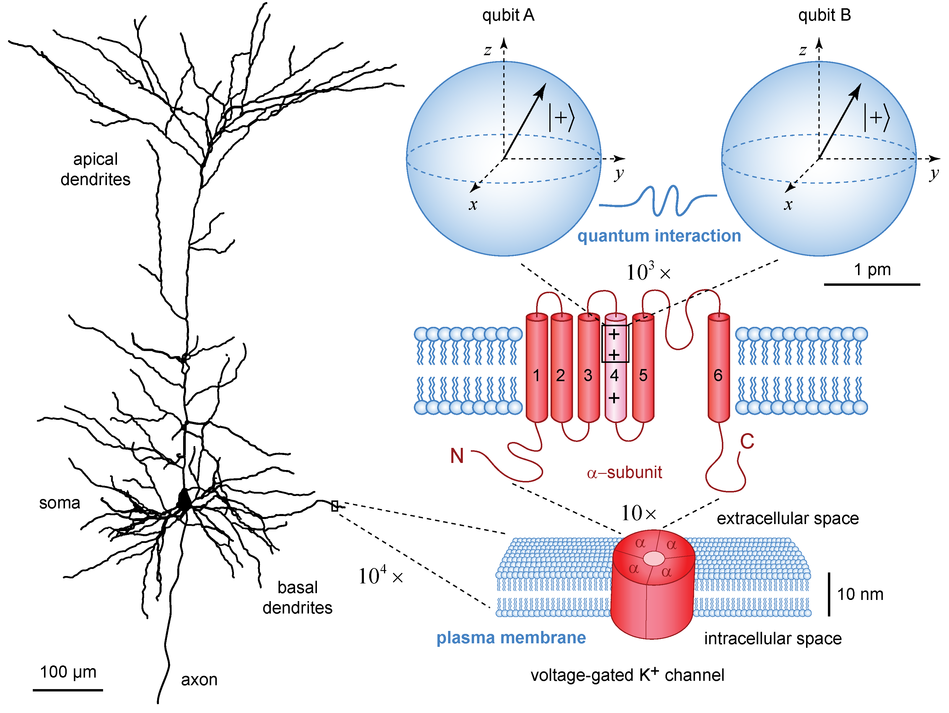
To substantiate the abstract quantum concepts in Hilbert space [43,44], we will construct a toy model whose quantum dynamics could be solved analytically and plotted for visual inspection. Because we will study quantum interactions, we need at least two quantum systems. Furthermore, because we would like the model to be biologically relevant (Figure 1), we will consider the quantum dynamics of electrons [45,46,47], which are elementary particles with spin-$\frac{1}{2}$ thereby acting as minimal quantum bits of information, or qubits [48]. The simplest possible composite quantum system that is capable of capturing the process of entanglement and decoherence is one composed of two non-identical interacting qubits in a uniform static magnetic field $\overrightarrow{B}$ aligned in the z-direction.

3.1. Hamiltonian of the Toy Model

Let ${\mathcal{H}}_A$ be the two-dimensional complex Hilbert space of the first qubit A and ${\mathcal{H}}_B$ be the two-dimensional complex Hilbert space of the second qubit B. Then according to the Dirac–von Neumann axioms of quantum mechanics [19,20], the composite two-qubit quantum system resides in a four-dimensional complex Hilbert space ${\mathcal{H}}_{AB}={\mathcal{H}}_A\otimes {\mathcal{H}}_B$, where ⊗ denotes the tensor product (also known as Kronecker product of matrices). The eigenvectors of the observable ${\widehat{S}}_{z,i}$ describing the spin component along the z-axis for the individual Hilbert spaces can be written as $\left\{{|\uparrow }_z{\rangle }_i{,|\downarrow }_z{\rangle }_i\right\}$ where $i=A,B$. The corresponding eigenvalues appear as scaling factors in the relations

$$\begin{array}{cc}\hfill {\widehat{S}}_{z,i}|& {\uparrow }_z{\rangle }_i=\frac{\hslash }{2}{|\uparrow }_z{\rangle }_i\hfill \end{array}$$

(3)

$$\begin{array}{cc}\hfill {\widehat{S}}_{z,i}|& {\downarrow }_z{\rangle }_i=-\frac{\hslash }{2}{|\downarrow }_z{\rangle }_i,\hfill \end{array}$$

(4)

where the reduced Planck constant is $\hslash =1.055\times {10}^{-34}$ J s. With the use of the Pauli spin matrices, ${\widehat{\sigma }}_x$, ${\widehat{\sigma }}_y$ and ${\widehat{\sigma }}_z$, we can define all three different spin components as ${\widehat{S}}_{x,i}=\frac{\hslash }{2}{\widehat{\sigma }}_x$, ${\widehat{S}}_{y,i}=\frac{\hslash }{2}{\widehat{\sigma }}_y$ and ${\widehat{S}}_{z,i}=\frac{\hslash }{2}{\widehat{\sigma }}_z$ in the respective Hilbert spaces ${\mathcal{H}}_A$ and ${\mathcal{H}}_B$.

In the composite four-dimensional complex Hilbert space ${\mathcal{H}}_{AB}$, we can explicitly write quantum states or quantum observables in matrix form using a chosen basis. For the description of the two-qubit toy model, we will adopt the spin $zz$ basis, $\left\{{|\uparrow }_z{\uparrow }_z{\rangle ,|\uparrow }_z{\downarrow }_z{\rangle ,|\downarrow }_z{\uparrow }_z{\rangle ,|\downarrow }_z{\downarrow }_z\rangle \right\}$, where for economy of notation we have used ordering from left to right to indicate which subsystem $i=A,B$ is referred to, namely

$$\begin{array}{cc}\hfill {|\uparrow }_z{\uparrow }_z\rangle & \equiv {|\uparrow }_z{\rangle }_A{|\uparrow }_z{\rangle }_B\hfill \end{array}$$

(5)

$$\begin{array}{cc}\hfill {|\uparrow }_z{\downarrow }_z\rangle & \equiv {|\uparrow }_z{\rangle }_A{|\downarrow }_z{\rangle }_B\hfill \end{array}$$

(6)

$$\begin{array}{cc}\hfill {|\downarrow }_z{\uparrow }_z\rangle & \equiv {|\downarrow }_z{\rangle }_A{|\uparrow }_z{\rangle }_B\hfill \end{array}$$

(7)

$$\begin{array}{cc}\hfill {|\downarrow }_z{\downarrow }_z\rangle & \equiv {|\downarrow }_z{\rangle }_A{|\downarrow }_z{\rangle }_B.\hfill \end{array}$$

(8)

Then, the individual spin observables in ${\mathcal{H}}_{AB}$ are given by product operators

$${\widehat{S}}_{x,A}=\frac{\hslash }{2}{\widehat{\sigma }}_x\otimes {\widehat{I}}_B=\frac{\hslash }{2}\left(\begin{array}{cc}0& 1\\ 1& 0\end{array}\right)\otimes \left(\begin{array}{cc}1& 0\\ 0& 1\end{array}\right)=\frac{\hslash }{2}\left(\begin{array}{cccc}0& 0& 1& 0\\ 0& 0& 0& 1\\ 1& 0& 0& 0\\ 0& 1& 0& 0\end{array}\right)$$

(9)

$${\widehat{S}}_{x,B}=\frac{\hslash }{2}{\widehat{I}}_A\otimes {\widehat{\sigma }}_x=\frac{\hslash }{2}\left(\begin{array}{cc}1& 0\\ 0& 1\end{array}\right)\otimes \left(\begin{array}{cc}0& 1\\ 1& 0\end{array}\right)=\frac{\hslash }{2}\left(\begin{array}{cccc}0& 1& 0& 0\\ 1& 0& 0& 0\\ 0& 0& 0& 1\\ 0& 0& 1& 0\end{array}\right)$$

(10)

$${\widehat{S}}_{y,A}=\frac{\hslash }{2}{\widehat{\sigma }}_y\otimes {\widehat{I}}_B=\frac{\hslash }{2}\left(\begin{array}{cc}0& -ı\\ ı& 0\end{array}\right)\otimes \left(\begin{array}{cc}1& 0\\ 0& 1\end{array}\right)=\frac{\hslash }{2}\left(\begin{array}{cccc}0& 0& -ı& 0\\ 0& 0& 0& -ı\\ ı& 0& 0& 0\\ 0& ı& 0& 0\end{array}\right)$$

(11)

$${\widehat{S}}_{y,B}=\frac{\hslash }{2}{\widehat{I}}_A\otimes {\widehat{\sigma }}_y=\frac{\hslash }{2}\left(\begin{array}{cc}1& 0\\ 0& 1\end{array}\right)\otimes \left(\begin{array}{cc}0& -ı\\ ı& 0\end{array}\right)=\frac{\hslash }{2}\left(\begin{array}{cccc}0& -ı& 0& 0\\ ı& 0& 0& 0\\ 0& 0& 0& -ı\\ 0& 0& ı& 0\end{array}\right)$$

(12)

$${\widehat{S}}_{z,A}=\frac{\hslash }{2}{\widehat{\sigma }}_z\otimes {\widehat{I}}_B=\frac{\hslash }{2}\left(\begin{array}{cc}1& 0\\ 0& -1\end{array}\right)\otimes \left(\begin{array}{cc}1& 0\\ 0& 1\end{array}\right)=\frac{\hslash }{2}\left(\begin{array}{cccc}1& 0& 0& 0\\ 0& 1& 0& 0\\ 0& 0& -1& 0\\ 0& 0& 0& -1\end{array}\right)$$

(13)

$${\widehat{S}}_{z,B}=\frac{\hslash }{2}{\widehat{I}}_A\otimes {\widehat{\sigma }}_z=\frac{\hslash }{2}\left(\begin{array}{cc}1& 0\\ 0& 1\end{array}\right)\otimes \left(\begin{array}{cc}1& 0\\ 0& -1\end{array}\right)=\frac{\hslash }{2}\left(\begin{array}{cccc}1& 0& 0& 0\\ 0& -1& 0& 0\\ 0& 0& 1& 0\\ 0& 0& 0& -1\end{array}\right).$$

(14)

The magnetic moments of the two qubits are ${\overrightarrow{\mu }}_1={\gamma }_1{\overrightarrow{S}}_1$ and ${\overrightarrow{\mu }}_2={\gamma }_2{\overrightarrow{S}}_2$, where the gyromagnetic ratios are ${\gamma }_1=g_1\frac{q_1}{2m_1}$ and ${\gamma }_2=g_2\frac{q_2}{2m_2}$, with g-factors $g_1$ and $g_2$, electric charges $q_1$ and $q_2$, and masses $m_1$ and $m_2$.

For a qubit that is realized by a spinning electron, we have

$$\overrightarrow{\mu }={\gamma }_e\overrightarrow{S}=g_e\frac{q_e}{2m_e}\overrightarrow{S}=g_e\frac{{\mu }_B}{\hslash }\overrightarrow{S},$$

(15)

where the electron g-factor is $g_e=-2.00231930436256$ and the Bohr magneton is ${\mu }_B=\frac{q_e\hslash }{2m_e}\approx 9.27\times {10}^{-24}$ J/Tesla.

If the internal Hamiltonians for each of the two qubits A and B are respectively

$$\begin{array}{cc}\hfill {\widehat{H}}_A& =-{\mu }_1·\overrightarrow{B}\hfill \end{array}$$

(16)

$$\begin{array}{cc}\hfill {\widehat{H}}_B& =-{\mu }_2·\overrightarrow{B}\hfill \end{array}$$

(17)

and the interaction between the two qubits is given by

$${\widehat{H}}_{\mathrm{int}}=\xi \left({\overrightarrow{S}}_1·{\overrightarrow{S}}_2\right)$$

(18)

we can write the total Hamiltonian as

$$\widehat{H}={\widehat{H}}_A+{\widehat{H}}_B+{\widehat{H}}_{\mathrm{int}}.$$

(19)

After substitution and expanding the inner products, we have

$$\begin{array}{cc}\hfill \widehat{H}& =-{\mu }_1·\overrightarrow{B}-{\mu }_2·\overrightarrow{B}+\xi \left({\overrightarrow{S}}_1·{\overrightarrow{S}}_2\right)\hfill \\ \hfill & ={\mathsf{\Omega }}_1{\overrightarrow{S}}_{z,A}+{\mathsf{\Omega }}_2{\overrightarrow{S}}_{z,B}+\xi \left({\widehat{S}}_{x,A}{\widehat{S}}_{x,B}+{\widehat{S}}_{y,A}{\widehat{S}}_{y,B}+{\widehat{S}}_{z,A}{\widehat{S}}_{z,B}\right)\hfill \\ \hfill & =\frac{\hslash }{2}{\mathsf{\Omega }}_1\left(\begin{array}{cccc}1& 0& 0& 0\\ 0& 1& 0& 0\\ 0& 0& -1& 0\\ 0& 0& 0& -1\end{array}\right)+\frac{\hslash }{2}{\mathsf{\Omega }}_2\left(\begin{array}{cccc}1& 0& 0& 0\\ 0& -1& 0& 0\\ 0& 0& 1& 0\\ 0& 0& 0& -1\end{array}\right)+\frac{{\hslash }^2}{4}\xi \left(\begin{array}{cccc}1& 0& 0& 0\\ 0& -1& 2& 0\\ 0& 2& -1& 0\\ 0& 0& 0& 1\end{array}\right)\hfill \\ \hfill & =\left(\begin{array}{cccc}{E}_{+}+E_s& 0& 0& 0\\ 0& E_{-}-E_s& 2E_s& 0\\ 0& 2E_s& -E_{-}-E_s& 0\\ 0& 0& 0& -E_{+}+E_s\end{array}\right),\hfill \end{array}$$

(20)

where $E_{+}=\frac{1}{2}\hslash \left({\mathsf{\Omega }}_1+{\mathsf{\Omega }}_2\right)$, $E_{-}=\frac{1}{2}\hslash \left({\mathsf{\Omega }}_1-{\mathsf{\Omega }}_2\right)$ and $E_s=\frac{{\hslash }^2}{4}\xi$. The corresponding angular frequencies are ${\omega }_{+}=\frac{1}{2}\left({\mathsf{\Omega }}_1+{\mathsf{\Omega }}_2\right)$, ${\omega }_{-}=\frac{1}{2}\left({\mathsf{\Omega }}_1-{\mathsf{\Omega }}_2\right)$ and ${\omega }_s=\frac{\hslash }{4}\xi$.

3.2. Energy Eigenstates and Eigenvalues of the Toy Model

The eigenvalues and eigenvectors of the Hamiltonian correspond to physical energies that enter in the general solution of the Schrödinger equation [21]. The energy eigenvalues of the concrete toy Hamiltonian (20) are found to be

$$\begin{array}{}\mathrm{(21)}& E_1\hfill & =E_{+}+E_s\hfill \mathrm{(22)}& E_2\hfill & =-E_s-\sqrt{E_{-}^2+4E_s^2}\hfill \mathrm{(23)}& E_3\hfill & =-E_s+\sqrt{E_{-}^2+4E_s^2}\hfill \mathrm{(24)}& E_4\hfill & =-E_{+}+E_s.\hfill \end{array}$$

Their corresponding energy eigenvectors expressed in the spin $zz$ basis are given by

$$\begin{array}{}\mathrm{(25)}& |E_1\rangle \hfill & ={|\uparrow }_z{\uparrow }_z\rangle \hfill \mathrm{(26)}& |E_2\rangle \hfill & =-C_1{|\uparrow }_z{\downarrow }_z\rangle +C_2{|\downarrow }_z{\uparrow }_z\rangle \hfill \mathrm{(27)}& |E_3\rangle \hfill & =C_2{|\uparrow }_z{\downarrow }_z\rangle +C_1{|\downarrow }_z{\uparrow }_z\rangle \hfill \mathrm{(28)}& |E_4\rangle \hfill & ={|\downarrow }_z{\downarrow }_z\rangle ,\hfill \end{array}$$

where for economy of notation we have set

$$\begin{array}{cc}\hfill C_1& =sin\left[\frac{1}{2}arccos\left(\frac{E_{-}}{\sqrt{E_{-}^2+4E_s^2}}\right)\right]=\frac{1}{\sqrt{2}}\sqrt{1-\frac{E_{-}}{\sqrt{E_{-}^2+4E_s^2}}}\hfill \end{array}$$

(29)

$$\begin{array}{cc}\hfill C_2& =cos\left[\frac{1}{2}arccos\left(\frac{E_{-}}{\sqrt{E_{-}^2+4E_s^2}}\right)\right]=\frac{1}{\sqrt{2}}\sqrt{1+\frac{E_{-}}{\sqrt{E_{-}^2+4E_s^2}}}.\hfill \end{array}$$

(30)

The mathematical relationship between eigenvectors and their eigenvalues allows for easy computation of the action of the Hamiltonian operator, namely

$$\widehat{H}|E_n\rangle =E_n|E_n\rangle .$$

(31)

Hence, if we express the initial composite two-qubit quantum state $|\mathsf{\Psi }\rangle$ in the energy basis

$$|\mathsf{\Psi }\rangle =\widehat{I}|\mathsf{\Psi }\rangle =\sum _n\widehat{\mathcal{P}}\left(E_n\right)|\mathsf{\Psi }\rangle =\sum _n|E_n\rangle \langle E_n|\mathsf{\Psi }\rangle =\sum _n{\alpha }_n|E_n\rangle ,$$

(32)

we can propagate it in time using the Schrödinger equation

$$ı\hslash \frac{\partial }{\partial t}|\mathsf{\Psi }\rangle =\widehat{H}|\mathsf{\Psi }\rangle =\widehat{H}\sum _n{\alpha }_n|E_n\rangle =\sum _n{E}_n{\alpha }_n|E_n\rangle .$$

(33)

Explicitly rewriting the quantum state in the energy basis gives a system of differential equations

$$ı\hslash \frac{\partial }{\partial t}\left(\begin{array}{c}{\alpha }_1\\ {\alpha }_2\\ ⋮\\ {\alpha }_n\end{array}\right)=\left(\begin{array}{c}{E}_1{\alpha }_1\\ E_2{\alpha }_2\\ ⋮\\ E_n{\alpha }_n\end{array}\right).$$

(34)

Before we solve these differential equations, we can divide both sides by $ı\hslash$ and work only with the angular frequencies

$$\frac{\partial }{\partial t}\left(\begin{array}{c}{\alpha }_1\\ {\alpha }_2\\ ⋮\\ {\alpha }_n\end{array}\right)=-ı\left(\begin{array}{c}{\omega }_1{\alpha }_1\\ {\omega }_2{\alpha }_2\\ ⋮\\ {\omega }_n{\alpha }_n\end{array}\right),$$

(35)

where ${\omega }_1=E_1/\hslash$, ${\omega }_2=E_2/\hslash$, …, ${\omega }_n=E_n/\hslash$. Quantum physicists usually take the approach of working in units in which $\hslash =1$, hence energy and angular frequency become equivalent by the Planck–Einstein relation $E=\hslash \omega$. However, our chosen approach is more general as it does not require fixing the physical units. Also, compared to energy, the angular frequencies are more appropriate for characterizing the dynamic timescale of the composite quantum system.

3.3. Quantum Dynamics of the State Vector

The solutions of the Schrödinger Equation (35) are easily found in the form

$${\alpha }_n\left(t\right)={\alpha }_n\left(0\right)e^{-ı{\omega }_{n}t},$$

(36)

with the immediate interpretation that ${\alpha }_n\left(0\right)$ is the initial quantum probability amplitude of the state $|E_n\rangle$ at $t=0$.

Then, the general solution of the time-dependent Schrödinger equation becomes

$$\begin{array}{}\mathrm{(37)}& |\mathsf{\Psi }(t)\rangle \hfill & =\sum _n{\alpha }_n\left(0\right)e^{-ı{\omega }_{n}t}|E_n\rangle \hfill \mathrm{(38)}& & ={\alpha }_1\left(0\right)e^{-ı{\omega }_{1}t}|E_1\rangle +{\alpha }_2\left(0\right)e^{-ı{\omega }_{2}t}|E_2\rangle +{\alpha }_3\left(0\right)e^{-ı{\omega }_{3}t}|E_3\rangle +{\alpha }_4\left(0\right)e^{-ı{\omega }_{4}t}|E_4\rangle ,\hfill \end{array}$$

where from Equations (21)–(24) we obtain

$$\begin{array}{}\mathrm{(39)}& {\omega }_1\hfill & ={\omega }_{+}+{\omega }_s\hfill \mathrm{(40)}& \hfill {\omega }_2& =-{\omega }_s-\sqrt{{\omega }_{-}^2+4{\omega }_s^2}\hfill \mathrm{(41)}& {\omega }_3\hfill & =-{\omega }_s+\sqrt{{\omega }_{-}^2+4{\omega }_s^2}\hfill \mathrm{(42)}& \hfill {\omega }_4& =-{\omega }_{+}+{\omega }_s.\hfill \end{array}$$

The coefficients of the energy eigenstates also can be fully re-written in terms of the angular frequencies

$$\begin{array}{cc}\hfill C_1& =\frac{1}{\sqrt{2}}\sqrt{1-\frac{{\omega }_{-}}{\sqrt{{\omega }_{-}^2+4{\omega }_s^2}}}\hfill \end{array}$$

(43)

$$\begin{array}{cc}\hfill C_2& =\frac{1}{\sqrt{2}}\sqrt{1+\frac{{\omega }_{-}}{\sqrt{{\omega }_{-}^2+4{\omega }_s^2}}}.\hfill \end{array}$$

(44)

Thus, the general quantum state $|\mathsf{\Psi }(t)\rangle$ at any time t is expressed as

$$\begin{array}{cc}\hfill |\mathsf{\Psi }(t)\rangle & ={\alpha }_1\left(0\right)e^{-ı{\omega }_{1}t}{|\uparrow }_z{\uparrow }_z\rangle -\left(C_1{\alpha }_2\left(0\right)e^{-ı{\omega }_{2}t}-C_2{\alpha }_3\left(0\right)e^{-ı{\omega }_{3}t}\right){|\uparrow }_z{\downarrow }_z\rangle \hfill \\ \hfill & +\left(C_2{\alpha }_2\left(0\right)e^{-ı{\omega }_{2}t}+C_1{\alpha }_3\left(0\right)e^{-ı{\omega }_{3}t}\right){|\downarrow }_z{\uparrow }_z\rangle +{\alpha }_4\left(0\right)e^{-ı{\omega }_{4}t}{|\downarrow }_z{\downarrow }_z\rangle .\hfill \end{array}$$

(45)

The initial energy quantum probability amplitudes can be further re-written in their exponential form as

$${\alpha }_i\left(0\right)=\left|{\alpha }_i\left(0\right)\right|e^{ı{\phi }_i},$$

(46)

where the principal arguments are

$${\phi }_i\equiv \mathrm{Arg}\left[{\alpha }_i\left(0\right)\right].$$

(47)

The quantum state $|\mathsf{\Psi }(t)\rangle$ describes what exists in the quantum world. The quantum state, however, is not an observable entity [49]. In order to determine what can be measured, we need to consider the expectation values of quantum observables.

4. Quantum Dynamic Timescale

To determine the relevant dynamic timescale, we need to account for Landauer’s principle, according to which there is a minimum possible amount of energy $E_{min}$ required to erase one bit of information [50] or to transmit one bit successfully across a noisy quantum channel affected by thermal noise [51,52]

$$E_{min}=k_{B}Tln2\approx 2.97\times {10}^{-21}\mathrm{J},$$

(48)

where $k_B=1.38\times {10}^{-23}$ J/K is the Boltzmann constant and $T=310$ K is the physiological body temperature of humans. From the Planck–Einstein relation $E=\hslash \omega$, we can determine the minimal angular frequency

$${\omega }_{min}=\frac{k_{B}Tln2}{\hslash }\approx 2.8\times {10}^{13}\mathrm{rad}/\mathrm{s}.$$

(49)

This means that there will be $\frac{{\omega }_{min}}{2\pi }\times {10}^{-12}\approx 4.5$ full rotations for time period of 1 ps. The time period for 1 full rotation is $\frac{2\pi }{{\omega }_{min}}\approx 0.22$ ps.

As an alternative calculation, consider the interaction of the Bohr magneton with an external magnetic field of 3 Tesla, which is routinely used for functional magnetic resonance imaging (fMRI) of the human brain, to obtain an interaction energy

$$\frac{1}{2}{g}_e{\mu }_{B}B\approx 2.78\times {10}^{-23}\mathrm{J},$$

(50)

that is about 100 times smaller than the Landauer’s limit. The corresponding angular frequency is

$${\mathsf{\Omega }}_1={\mathsf{\Omega }}_2=\frac{g_e{\mu }_{B}B}{2\hslash }\approx 2.64\times {10}^{11}\mathrm{rad}/\mathrm{s}.$$

(51)

This means that there will be $\frac{{\mathsf{\Omega }}_1}{2\pi }\times {10}^{-10}\approx 4.2$ full rotations for time period of 100 ps. The time period for 1 full rotation is $\frac{2\pi }{{\omega }_{\mathrm{int}}}\approx 23.8$ ps. One possible interpretation of the latter result is that the MRI experimental technique is by a factor of ≈100 slower that the predicted quantum characteristic time of neural processes related to consciousness.

The main conclusion is that for typical energies that are comparable to the thermal energy, the rotation of the state vector in Hilbert space occurs with time period at a subpicosecond timescale. For energies that are an order of magnitude lower than the thermal energy, the dynamic timescale is picoseconds, for energies that are two orders of magnitude lower than the thermal energy, the dynamic timescale is tens of picoseconds, and so on. Therefore, the Planck–Einstein relation $E=\hslash \omega$ that appears in the Schrödinger equation fixes the dynamic timescale of quantum processes to picosecond timescale or faster, which is in the realm of quantum chemistry [8,24]. For complex biomolecules such as proteins, which catalyze life-sustaining physiological activities, key functional role is played by hydrogen bonds whose energy is an order of magnitude lower compared to covalent bonds. Consequently, the quantum transport of energy in protein $\alpha$-helices due to conformational bending of hydrogen bonded peptide groups occurs at picosecond timescale [53,54,55], as opposed to femtosecond electron transport due to destruction or creation of covalent bonds [56,57,58,59,60]. Quantum theories of consciousness that require operation at longer timescales, such as milliseconds, are incompatible with the essentials established by the Planck–Einstein relation and the Schrödinger equation.

Here, we would like to emphasize that there are contrived methods based on quantum beats that could realize destructive quantum interference in order to slow down the quantum dynamics of the expectation value of some quantum observables, however, those methods are not evolutionary plausible as they reduce the computational power of the brain. To appreciate the meaning of this criticism, consider the operation of computer processors realized on silicon chips: a processor that operates at MHz (microsecond timescale) can perform only ${10}^6$ operations per second, whereas a processor that operates at GHz (nanosecond timescale) can perform ${10}^9$ operations per second. The faster the processor is, the more computational power it has. That is why modern computing technologies aim toward processors operating at THz (picosecond timescale), where quantum effects become dominant, rather than the slower timescale of milliseconds or even seconds, where the computation can be performed manually e.g., by sliding beads on abacus.

5. Quantum Entanglement

Quantum entanglement entails interdependence between different component subsystems, which form a composite quantum system [61]. Although the quantum entanglement could be manifested in the form of correlations between observable outcomes, the converse is not true, namely the lack of correlations between observable outcomes does not imply the lack of entanglement. This is because quantum entanglement is defined for the quantum state, which is a vector in Hilbert space, whereas the probabilities for occurrence of definite measurement outcomes pertain to quantum observables, which are operators on the Hilbert space.

Incompatible (non-commuting) observables cannot be measured simultaneously with a single experimental setting of the measurement apparatus. This means that in the act of quantum measurement only a set of compatible (commuting) quantum observables can be determined to have a definite value. Those quantum observables that are not measured do not have a definite value and consequently there are no actual measurement outcomes from which could be extracted correlations. If one is careful to distinguish between what is actual and what is counterfactual, quantum mechanics allows for exact prediction of the possible correlations that would have been observed had the necessary quantum measurements been performed.

Definition 1.

(Separable state) A bipartite composite quantum state $|\mathsf{\Psi }\rangle \in {\mathcal{H}}_A\otimes {\mathcal{H}}_B$ is called separable if and only if it can be written as a tensor product [62]

$$|\mathsf{\Psi }\rangle ={|\psi \rangle }_A\otimes {|\psi \rangle }_B.$$

(52)

Definition 2.

(Entangled state) A bipartite composite quantum state $|\mathsf{\Psi }\rangle \in {\mathcal{H}}_A\otimes {\mathcal{H}}_B$ is called entangled if and only if it cannot be written as a tensor product [62]

$$|\mathsf{\Psi }\rangle \ne {|\psi \rangle }_A\otimes {|\psi \rangle }_B.$$

(53)

Theorem 1.

(Schmidt decomposition) Let$\left\{{|i\rangle }_A\right\}$be a basis for ${\mathcal{H}}_A$ and$\left\{{|j\rangle }_B\right\}$be a basis for ${\mathcal{H}}_B$. Then, every bipartite composite quantum state $|\mathsf{\Psi }\rangle \in {\mathcal{H}}_A\otimes {\mathcal{H}}_B$ can be expressed in $\left\{{|i\rangle }_A{|j\rangle }_B\right\}$ basis as follows

$$|\mathsf{\Psi }\rangle =\sum _i\sum _j{c}_{ij}{|i\rangle }_A{|j\rangle }_B.$$

(54)

Next, construct the matrix $\widehat{C}=\left(c_{ij}\right)$ and perform singular value decomposition in the form

$$\widehat{C}=\widehat{U}\widehat{\mathsf{\Lambda }}{\widehat{V}}^{†},$$

(55)

where $\widehat{U}$ and ${\widehat{V}}^{†}$ are unitary matrices, and $\widehat{\mathsf{\Lambda }}$ is a diagonal matrix with non-negative singular values sorted in descending order ${\lambda }_1\ge {\lambda }_2\ge \dots \ge {\lambda }_s\ge 0$ also referred to as Schmidt coefficients. Thus, the bipartite composite quantum state becomes

$$|\mathsf{\Psi }\rangle =\sum _s{\lambda }_s{|\psi \rangle }_A\otimes {|\psi \rangle }_B,$$

(56)

where ${|\psi \rangle }_A=\widehat{U}{|i\rangle }_A$ and ${|\psi \rangle }_B={\widehat{V}}^{†}{|j\rangle }_B$ is the Schmidt basis [63]. The state is entangled if its Schmidt rank is greater than 1. Otherwise, the state is separable.

Theorem 2.

The singular values of a Hermitian matrix $\widehat{A}={\widehat{A}}^{†}$ are the absolute values of the eigenvalues of $\widehat{A}$.

Proof. 

Every Hermitian matrix has a complete set of eigenvectors, and all of its eigenvalues are real. This allows spectral decomposition

$$\widehat{A}=\widehat{U}\widehat{\mathsf{\Lambda }}{\widehat{U}}^{†},$$

(57)

where $\widehat{U}$ is unitary matrix and $\widehat{\mathsf{\Lambda }}={\widehat{\mathsf{\Lambda }}}^{†}$ is a diagonal matrix with real entries. Decompose the diagonal matrix as $\widehat{\mathsf{\Lambda }}=\left|\widehat{\mathsf{\Lambda }}\right|\mathrm{sign}\widehat{\mathsf{\Lambda }}$. The matrix ${\widehat{V}}^{†}=\mathrm{sign}\widehat{\mathsf{\Lambda }}{\widehat{U}}^{†}$ is unitary because ${\widehat{U}}^{†}$ is unitary. Therefore, the singular value decomposition of $\widehat{A}$ is

$$\widehat{A}=\widehat{U}\left|\widehat{\mathsf{\Lambda }}\right|{\widehat{V}}^{†}.$$

(58)

□

Definition 3.

The entanglement number $e\left(\mathsf{\Psi }\right)$ of a quantum state $|\mathsf{\Psi }\rangle$ is determined by the Schmidt coefficients using the formula [64]

$$e\left(\mathsf{\Psi }\right)=\sqrt{1-\sum _s{\lambda }_s^4}.$$

(59)

Theorem 3.

The Hermitian matrix $\widehat{C}{\widehat{C}}^{†}$ is positive semidefinite, namely $\langle x|\widehat{C}{\widehat{C}}^{†}|x\rangle \ge 0$ for all vectors x. The eigenvalues of the Hermitian matrix $\widehat{C}{\widehat{C}}^{†}=\widehat{U}\widehat{\mathsf{\Lambda }}{\widehat{V}}^{†}\widehat{V}\widehat{\mathsf{\Lambda }}{\widehat{U}}^{†}=\widehat{U}{\widehat{\mathsf{\Lambda }}}^2{\widehat{U}}^{†}$ are equal to ${\lambda }_s^2$. Therefore, an efficient way to compute the entanglement number without recourse to singular value decomposition is to use [64]

$$e\left(\mathsf{\Psi }\right)=\sqrt{1-Tr\left(\widehat{C}{\widehat{C}}^{†}\widehat{C}{\widehat{C}}^{†}\right)}.$$

(60)

The entanglement number could be normalized in the interval $[0,1]$ as follows

$$\tilde{e}\left(\mathsf{\Psi }\right)=\frac{e\left(\mathsf{\Psi }\right)}{e{\left(\mathsf{\Psi }\right)}_{max}},$$

(61)

where $e{\left(\mathsf{\Psi }\right)}_{max}$ is the maximal possible value, which is determined by the dimension n of the Hilbert space of the smallest subsystem, namely $n=min\left[d\left({\mathcal{H}}_A\right),d\left({\mathcal{H}}_B\right)\right]$. In the maximally entangled state, the Schmidt decomposition has n eigenvalues equal to $\frac{1}{\sqrt{n}}$, resulting in

$$e{\left(\mathsf{\Psi }\right)}_{max}=\sqrt{1-n\frac{1}{n^2}}=\sqrt{\frac{n-1}{n}}.$$

(62)

The normalized quantum entanglement number $e\left(\mathsf{\Psi }\right)$ in the toy model could be computed from the eigenvalues of $\widehat{C}{\widehat{C}}^{†}$ to be

$$\begin{array}{cc}\hfill \tilde{e}\left(\mathsf{\Psi }\right)& =2\{\left|{\alpha }_1^2\left(0\right){\alpha }_4^2\left(0\right)\right|+\left|{\alpha }_2^2\left(0\right){\alpha }_3^2\left(0\right)\right|+C_1^2{C}_2^2\left(\left|{\alpha }_2^4\left(0\right)\right|-4\left|{\alpha }_2^2\left(0\right){\alpha }_3^2\left(0\right)\right|+\left|{\alpha }_3^4\left(0\right)\right|\right)\hfill \\ \hfill & -2C_{+}{C}_{-}\left|{\alpha }_1\left(0\right){\alpha }_2\left(0\right){\alpha }_3\left(0\right){\alpha }_4\left(0\right)\right|cos\left[\left({\omega }_1-{\omega }_2-{\omega }_3+{\omega }_4\right)t-{\phi }_1+{\phi }_2+{\phi }_3-{\phi }_4\right]\hfill \\ \hfill & +2C_1{C}_2\left|{\alpha }_1\left(0\right){\alpha }_2^2\left(0\right){\alpha }_4\left(0\right)\right|cos\left[\left({\omega }_1-2{\omega }_2+{\omega }_4\right)t-{\phi }_1+2{\phi }_2-{\phi }_4\right]\hfill \\ \hfill & -2C_1{C}_2\left|{\alpha }_1\left(0\right){\alpha }_3^2\left(0\right){\alpha }_4\left(0\right)\right|cos\left[\left({\omega }_1-2{\omega }_3+{\omega }_4\right)t-{\phi }_1+2{\phi }_3-{\phi }_4\right]\hfill \\ \hfill & -2C_1{C}_2{C}_{+}{C}_{-}\left(\left|{\alpha }_2^3\left(0\right){\alpha }_3\left(0\right)\right|-\left|{\alpha }_2\left(0\right){\alpha }_3^3\left(0\right)\right|\right)cos\left[\left({\omega }_2-{\omega }_3\right)t-{\phi }_2+{\phi }_3\right]\hfill \\ \hfill & -2C_1^2{C}_2^2\left|{\alpha }_2^2\left(0\right){\alpha }_3^2\left(0\right)\right|cos\left[2\left({\omega }_2-{\omega }_3\right)t-2\left({\phi }_2-{\phi }_3\right)\right]{\}}^{\frac{1}{2}}.\hfill \end{array}$$

(63)

6. Quantum Coherence

Quantum coherence and decoherence are frequently mentioned in discussions on the feasibility of quantum approaches to consciousness [25,65]. Because the visibility of quantum interference patterns requires quantum superpositions [66,67], a careless wording may say that quantum coherence is indicative of present quantum superpositions, whereas decoherence is indicative of absent quantum superpositions. Unfortunately, such statements cannot be literally correct and would appear to be based on misunderstanding the vector nature of quantum states. Mathematically, a vector can always be decomposed into a superposition of other vectors, which means that the concept of quantum superposition is not an absolute property, but a basis-dependent one [8]. Therefore, it is meaningless to talk about the presence or absence of quantum superpositions without explicitly stating the basis in which those superpositions are considered.

Definition 4.

(Quantum coherence) The ${\ell }_1$ norm of coherence $\mathcal{C}$ is a basis-dependent quantitative measure of quantum coherence of an $n\times n$ dimensional density matrix $\widehat{\rho }$ defined with the use of the sum of all off-diagonal moduli [68]

$$\mathcal{C}=\frac{1}{n-1}\sum _{i\ne j}\left|{\rho }_{ij}\right|.$$

(64)

The quantum coherence is bounded in the interval $0\le \mathcal{C}\le 1$.

Example 1.

Consider a qubit in the state ${|\uparrow }_z\rangle$. The density matrix of the qubit in spin z basis is

$$\widehat{\rho }={|\uparrow }_z{\rangle \langle \uparrow }_z|=\left(\begin{array}{cc}1& 0\end{array}\right)\left(\begin{array}{c}1\\ 0\end{array}\right)=\left(\begin{array}{cc}1& 0\\ 0& 0\end{array}\right).$$

(65)

All off-diagonal elements of the density matrix $\widehat{\rho }$ expressed in spin z basis are zero, hence $\mathcal{C}=0$, indicating that the state is not superposed in that basis. However, the same density matrix re-written in spin x basis becomes

$$\widehat{\rho }=\frac{1}{\sqrt{2}}\left({|\uparrow }_x{\rangle +|\downarrow }_x\rangle \right)\frac{1}{\sqrt{2}}\left({\langle \uparrow }_x{|+\langle \downarrow }_x|\right)=\frac{1}{2}\left(\begin{array}{cc}1& 1\end{array}\right)\left(\begin{array}{c}1\\ 1\end{array}\right)=\frac{1}{2}\left(\begin{array}{cc}1& 1\\ 1& 1\end{array}\right).$$

(66)

All off-diagonal elements of the density matrix $\widehat{\rho }$ expressed in spin x basis are $\frac{1}{2}$, hence $\mathcal{C}=1$, indicating that the state is maximally superposed in that basis.

It should be emphasized that the disappearance of quantum coherence merely by change of basis of a pure state [69] is not the main physical phenomenon studied by decoherence theory. Instead, decoherence refers to the loss of quantum purity and conversion of pure quantum states into mixed quantum states [70,71,72,73]. In this latter process, the coherent quantum superpositions, which can manifest visible quantum interference patterns under suitable choice of measurement basis, become converted into incoherent quantum superpositions, which cannot manifest visible quantum interference patterns. In general, the loss of visibility of interference patterns is not abrupt, but occurs gradually with the loss of quantum purity.

Definition 5.

(Quantum purity) The quantum purity γ of an $n\times n$ dimensional density matrix $\widehat{\rho }$ is defined as

$$\gamma =Tr\left({\widehat{\rho }}^2\right).$$

(67)

The quantum purity is bounded in the interval $\frac{1}{n}\le \gamma \le 1$.

Example 2.

A maximally mixed state with minimal purity $\gamma =\frac{1}{2}$ is realized by a qubit with density matrix

$$\widehat{\rho }=\frac{1}{2}\left({|\uparrow }_z{\rangle \langle \uparrow }_z{|+|\downarrow }_z{\rangle \langle \downarrow }_z|\right)=\frac{1}{2}\left({|\uparrow }_x{\rangle \langle \uparrow }_x{|+|\downarrow }_x{\rangle \langle \downarrow }_x|\right)=\frac{1}{2}\left(\begin{array}{cc}1& 0\\ 0& 1\end{array}\right).$$

(68)

The maximally mixed state is incoherent in every basis, meaning that the ${\ell }_1$ norm of coherence $\mathcal{C}$ is zero in every basis. As a result, quantum measurement in any basis will find the spin with equal probability being in either of the two possible directions, up or down. Furthermore, quantum superpositions may still be present, even though the maximally mixed state will not manifest visible quantum interference patterns in any basis. For that latter reason, such quantum superpositions are called incoherent.

To understand where the incoherent quantum superpositions reside, we have to consider the quantum mechanical concept of purification.

Definition 6.

(Purification) Every mixed state given by a density matrix $\widehat{\rho }={\sum }_i{p}_i|i\rangle \langle i|$ acting on finite-dimensional Hilbert space ${\mathcal{H}}_A$ with basis $\left\{|i\rangle \right\}$ can be viewed as the reduced state of some pure state $|\mathsf{\Psi }\rangle \in {\mathcal{H}}_A\otimes {\mathcal{H}}_B$, where ${\mathcal{H}}_B$ is another copy of ${\mathcal{H}}_A$ with basis $\left\{|i^{\prime }\rangle \right\}$.

Proof. 

Every density matrix $\widehat{\rho }\in {\mathcal{H}}_A$ can be spectrally decomposed in terms of its eigenvalues $p_i$ and corresponding set of orthonormal eigenvectors $\left\{|i\rangle \right\}$. Working with the basis $\left\{|i\rangle \right\}$ massively simplifies the calculations because the density matrix $\widehat{\rho }$ becomes diagonal in that basis. Then, consider the state $|\mathsf{\Psi }\rangle ={\sum }_i\sqrt{p_i}|i\rangle \otimes |i^{\prime }\rangle$. Explicit calculation of the partial trace gives

$$\begin{array}{cc}\hfill \widehat{\rho }& ={\mathrm{Tr}}_B|\mathsf{\Psi }\rangle \langle \mathsf{\Psi }|\hfill \\ \hfill & ={\mathrm{Tr}}_B\left(\sum _i\sqrt{p_i}|i\rangle \otimes |i^{\prime }\rangle \sum _j\sqrt{p_j}\langle j|\otimes \langle j^{\prime }|\right)\hfill \\ \hfill & ={\mathrm{Tr}}_B\sum _i\sum _j\sqrt{p_i{p}_j}|i\rangle \langle j|\otimes |i^{\prime }\rangle \langle j^{\prime }|\hfill \\ \hfill & =\sum _i\sum _j{\delta }_{ij}\sqrt{p_i{p}_j}|i\rangle \langle j|\hfill \\ \hfill & =\sum _i{p}_i|i\rangle \langle i|.\hfill \end{array}$$

(69)

□

Example 3.

Consider two qubits A and B comprising the pure maximally entangled (anti-correlated) quantum state

$${|\mathsf{\Psi }\rangle }_{AB}=\frac{1}{\sqrt{2}}\left({|\uparrow }_z{\downarrow }_z{\rangle +|\downarrow }_z{\uparrow }_z\rangle \right).$$

(70)

The composite density matrix is pure

$${\widehat{\rho }}_{AB}={\widehat{\rho }}_{AB}^2=\frac{1}{2}\left(\begin{array}{cccc}0& 0& 0& 0\\ 0& 1& 1& 0\\ 0& 1& 1& 0\\ 0& 0& 0& 0\end{array}\right),$$

(71)

whereas the reduced density matrices of each qubit are maximally mixed

$${\widehat{\rho }}_A={Tr}_B\left({\widehat{\rho }}_{AB}\right)={\widehat{\rho }}_B={Tr}_A\left({\widehat{\rho }}_{AB}\right)=\frac{1}{2}\left(\begin{array}{cc}1& 0\\ 0& 1\end{array}\right).$$

(72)

Thus, the quantum superposition is seen as non-zero off-diagonal elements only in the composite density matrix ${\widehat{\rho }}_{AB}$, but not in the reduced density matrices ${\widehat{\rho }}_A$ and ${\widehat{\rho }}_B$.

Example 4.

Consider two qubits A and B comprising the pure maximally entangled (correlated) quantum state

$${|\mathsf{\Psi }\rangle }_{AB}=\frac{1}{\sqrt{2}}\left({|\uparrow }_z{\uparrow }_z{\rangle +|\downarrow }_z{\downarrow }_z\rangle \right).$$

(73)

Again, the composite density matrix is pure

$${\widehat{\rho }}_{AB}={\widehat{\rho }}_{AB}^2=\frac{1}{2}\left(\begin{array}{cccc}1& 0& 0& 1\\ 0& 0& 0& 0\\ 0& 0& 0& 0\\ 1& 0& 0& 1\end{array}\right),$$

(74)

whereas the reduced density matrices of each qubit are maximally mixed

$${\widehat{\rho }}_A={\mathit{Tr}}_B\left({\widehat{\rho }}_{AB}\right)={\widehat{\rho }}_B={\mathit{Tr}}_A\left({\widehat{\rho }}_{AB}\right)=\frac{1}{2}\left(\begin{array}{cc}1& 0\\ 0& 1\end{array}\right).$$

(75)

The reduced density matrices ${\widehat{\rho }}_A$ and ${\widehat{\rho }}_B$ are exactly the same as in the case when the composite state is given by (70). Comparison of the the composite states (70) and (73) shows that the measurement outcomes of the z-components of the two spins will be correlated or anti-correlated, respectively. Therefore, knowing only the reduced density matrices of the components does not provide a complete description of the composite system, whereas knowing the composite state vector does.

In the context of decoherence theory, quantum coherence is used with the intended meaning of maximal purity. Keeping this clarification in mind, it could be said that the composite two-qubit system is quantum coherent because its purity is maximal, $\gamma =1$, whereas each of the component qubits is incoherent because its purity is minimal, $\gamma =\frac{1}{2}$. Thus, quantum entanglement leads to decoherence and the two processes go hand by hand. Conversely, the two component qubits cannot be individually maximally coherent (pure) and quantum entangled at the same time. Instead, if each of the two qubits is in a pure state, then the composite state is separable.

Example 5.

Consider each of the two qubits A and B being in coherent quantum superposition $\frac{1}{\sqrt{2}}\left({|\uparrow }_z{\rangle +|\downarrow }_z\rangle \right)$. The composite density matrix is pure

$${\widehat{\rho }}_{AB}={\widehat{\rho }}_{AB}^2=\frac{1}{4}\left(\begin{array}{cccc}1& 1& 1& 1\\ 1& 1& 1& 1\\ 1& 1& 1& 1\\ 1& 1& 1& 1\end{array}\right)$$

(76)

and the reduced density matrices of each qubit are also pure

$${\widehat{\rho }}_A={\widehat{\rho }}_A^2={\mathit{Tr}}_B\left({\widehat{\rho }}_{AB}\right)={\widehat{\rho }}_B={\widehat{\rho }}_B^2={\mathit{Tr}}_A\left({\widehat{\rho }}_{AB}\right)=\frac{1}{2}\left(\begin{array}{cc}1& 1\\ 1& 1\end{array}\right).$$

(77)

The separability of the composite state follows from the purity of the components

$${|\mathsf{\Psi }\rangle }_{AB}=\frac{1}{\sqrt{2}}\left({|\uparrow }_z{\rangle +|\downarrow }_z\rangle \right)\otimes \frac{1}{\sqrt{2}}\left({|\uparrow }_z{\rangle +|\downarrow }_z\rangle \right)={|\uparrow }_x{\rangle \otimes |\uparrow }_x\rangle .$$

(78)

From the preceding examples, it should be clear that quantum mechanics contains two very different kinds of relationships between composite systems and component systems. For separable states, both the composite system and the component systems have pure quantum states. This implies that it is possible to write state vectors for both the composite system and the component systems. For quantum entangled states, it is only the composite system that has a pure quantum state, whereas the component systems are necessarily described by mixed quantum states. Because mixed quantum states can only be represented in the form of a density matrix, but not a quantum state vector, this implies that the components of quantum entangled states cannot be completely described in isolation. Indeed, the reduced density matrices that describe the components of quantum entangled states can be used only for computing the quantum probabilities of outcomes from local measurements performed upon the given component. However, the reduced density matrices are useless for computing existing correlations between different components [8].

7. Measurement of Quantum Observables

So far, we have discussed the importance of the state vector $|\mathsf{\Psi }(t)\rangle$ of the composite system and have solved the Schrödinger equation for the two-qubit toy model. Although, the state vector $|\mathsf{\Psi }(t)\rangle$ is not an observable [49], it allows us to determine the expectation values of any physical observable $\widehat{A}$ that could be measured at any point in time t. The important thing to keep in mind is that non-commuting quantum observables are incompatible with each other and cannot be measured at the same time. This means that without knowing which observable is actually measured, the quantum dynamics of the expectation value of any quantum observable $\langle \widehat{A}\rangle =\langle \mathsf{\Psi }\left(t\right)|\widehat{A}|\mathsf{\Psi }\left(t\right)\rangle$ is to be considered as counterfactual, namely, it describes probability distributions of physical events that could have happened provided that the quantum observable $\widehat{A}$ were measured. Thus, quantum observables do not necessarily reflect what exists, but only what could be observed [23,24].

7.1. Quantum Observables in Spin $zz$ Basis

The probabilities for measuring the composite system in each of the spin $zz$ basis states from the set $\left\{{|\uparrow }_z{\uparrow }_z{\rangle ,|\uparrow }_z{\downarrow }_z{\rangle ,|\downarrow }_z{\uparrow }_z{\rangle ,|\downarrow }_z{\downarrow }_z\rangle \right\}$ are given by the expectation values of the corresponding projection operators according to the Born rule [74], namely

$$\begin{array}{cc}\hfill \mathrm{Prob}\left({\uparrow }_z{\uparrow }_z\right)& =\langle \mathsf{\Psi }\left(t\right)|\widehat{\mathcal{P}}\left({\uparrow }_z{\uparrow }_z\right)|\mathsf{\Psi }\left(t\right)\rangle ={\langle \mathsf{\Psi }\left(t\right)|\uparrow }_z{\uparrow }_z{\rangle \langle \uparrow }_z{\uparrow }_z|\mathsf{\Psi }\left(t\right)\rangle ={\left|\langle {\uparrow }_z{\uparrow }_z|\mathsf{\Psi }\left(t\right)\rangle \right|}^2\hfill \end{array}$$

(79)

$$\begin{array}{cc}\hfill \mathrm{Prob}\left({\uparrow }_z{\downarrow }_z\right)& =\langle \mathsf{\Psi }\left(t\right)|\widehat{\mathcal{P}}\left({\uparrow }_z{\downarrow }_z\right)|\mathsf{\Psi }\left(t\right)\rangle ={\langle \mathsf{\Psi }\left(t\right)|\uparrow }_z{\downarrow }_z{\rangle \langle \uparrow }_z{\downarrow }_z|\mathsf{\Psi }\left(t\right)\rangle ={\left|\langle {\uparrow }_z{\downarrow }_z|\mathsf{\Psi }\left(t\right)\rangle \right|}^2\hfill \end{array}$$

(80)

$$\begin{array}{cc}\hfill \mathrm{Prob}\left({\downarrow }_z{\uparrow }_z\right)& =\langle \mathsf{\Psi }\left(t\right)|\widehat{\mathcal{P}}\left({\downarrow }_z{\uparrow }_z\right)|\mathsf{\Psi }\left(t\right)\rangle ={\langle \mathsf{\Psi }\left(t\right)|\downarrow }_z{\uparrow }_z{\rangle \langle \downarrow }_z{\uparrow }_z|\mathsf{\Psi }\left(t\right)\rangle ={\left|\langle {\downarrow }_z{\uparrow }_z|\mathsf{\Psi }\left(t\right)\rangle \right|}^2\hfill \end{array}$$

(81)

$$\begin{array}{cc}\hfill \mathrm{Prob}\left({\downarrow }_z{\downarrow }_z\right)& =\langle \mathsf{\Psi }\left(t\right)|\widehat{\mathcal{P}}\left({\downarrow }_z{\downarrow }_z\right)|\mathsf{\Psi }\left(t\right)\rangle ={\langle \mathsf{\Psi }\left(t\right)|\downarrow }_z{\downarrow }_z{\rangle \langle \downarrow }_z{\downarrow }_z|\mathsf{\Psi }\left(t\right)\rangle ={\left|\langle {\downarrow }_z{\downarrow }_z|\mathsf{\Psi }\left(t\right)\rangle \right|}^2.\hfill \end{array}$$

(82)

Explicit calculation for the observable quantum probabilities gives

$$\begin{array}{}\mathrm{(83)}& \mathrm{Prob}\left({\uparrow }_z{\uparrow }_z\right)\hfill & ={\left|{\alpha }_1\left(0\right)\right|}^2\hfill \mathrm{(84)}& \mathrm{Prob}\left({\uparrow }_z{\downarrow }_z\right)\hfill & =C_1^2{\left|{\alpha }_2\left(0\right)\right|}^2-2C_1{C}_2\left|{\alpha }_2\left(0\right){\alpha }_3\left(0\right)\right|cos\left[\left({\omega }_2-{\omega }_3\right)t-{\phi }_2+{\phi }_3\right]+C_2^2{\left|{\alpha }_3\left(0\right)\right|}^2\hfill \mathrm{(85)}& \mathrm{Prob}\left({\downarrow }_z{\uparrow }_z\right)\hfill & =C_2^2{\left|{\alpha }_2\left(0\right)\right|}^2+2C_1{C}_2\left|{\alpha }_2\left(0\right){\alpha }_3\left(0\right)\right|cos\left[\left({\omega }_2-{\omega }_3\right)t-{\phi }_2+{\phi }_3\right]+C_1^2{\left|{\alpha }_3\left(0\right)\right|}^2\hfill \mathrm{(86)}& \mathrm{Prob}\left({\downarrow }_z{\downarrow }_z\right)\hfill & ={\left|{\alpha }_4\left(0\right)\right|}^2.\hfill \end{array}$$

It is easy to see that the four quantum probabilities sum up to unity since $C_1^2+C_2^2=1$ and ${\sum }_n{\left|{\alpha }_n\left(0\right)\right|}^2=1$.

In order to perform computer simulations, one can plug in directly different quantum probability amplitudes ${\alpha }_n\left(0\right)$ for the initial superposition of energy states $|\mathsf{\Psi }\left(0\right)\rangle ={\sum }_n{\alpha }_n\left(0\right)|E_n\rangle$ and then observe the quantum dynamics that follows. In the case when the initial quantum state $|\mathsf{\Psi }(0)\rangle$ is given in a different basis, such as an eigenvector of the evolving quantum observable, then one first needs to determine the initial quantum probability amplitudes ${\alpha }_n\left(0\right)$ for the energy states using inner products

$$|\mathsf{\Psi }\left(0\right)\rangle =\widehat{I}|\mathsf{\Psi }\left(0\right)\rangle =\sum _n|E_n\rangle \langle E_n|\mathsf{\Psi }\left(0\right)\rangle =\sum _n{\alpha }_n\left(0\right)|E_n\rangle$$

(87)

and then proceed with the computer simulation. As an explicit example, we present the initial energy quantum probability amplitudes for each of the spin $zz$ basis states in the energy basis

$$\begin{array}{}\mathrm{(88)}& {|\uparrow }_z{\uparrow }_z\rangle \hfill & =\hfill & |E_1\rangle \hfill \mathrm{(89)}& {|\uparrow }_z{\downarrow }_z\rangle \hfill & =\hfill & -C_1|E_2\rangle +C_2|E_3\rangle \hfill \mathrm{(90)}& {|\downarrow }_z{\uparrow }_z\rangle \hfill & =\hfill & C_2|E_2\rangle +C_1|E_3\rangle \hfill \mathrm{(91)}& {|\downarrow }_z{\downarrow }_z\rangle \hfill & =\hfill & |E_4\rangle .\hfill \end{array}$$

Once we have the initial quantum probability amplitudes in the energy basis, we can plot the quantum dynamics of the expectation values of the quantum observables given in Equations (83)–(86).

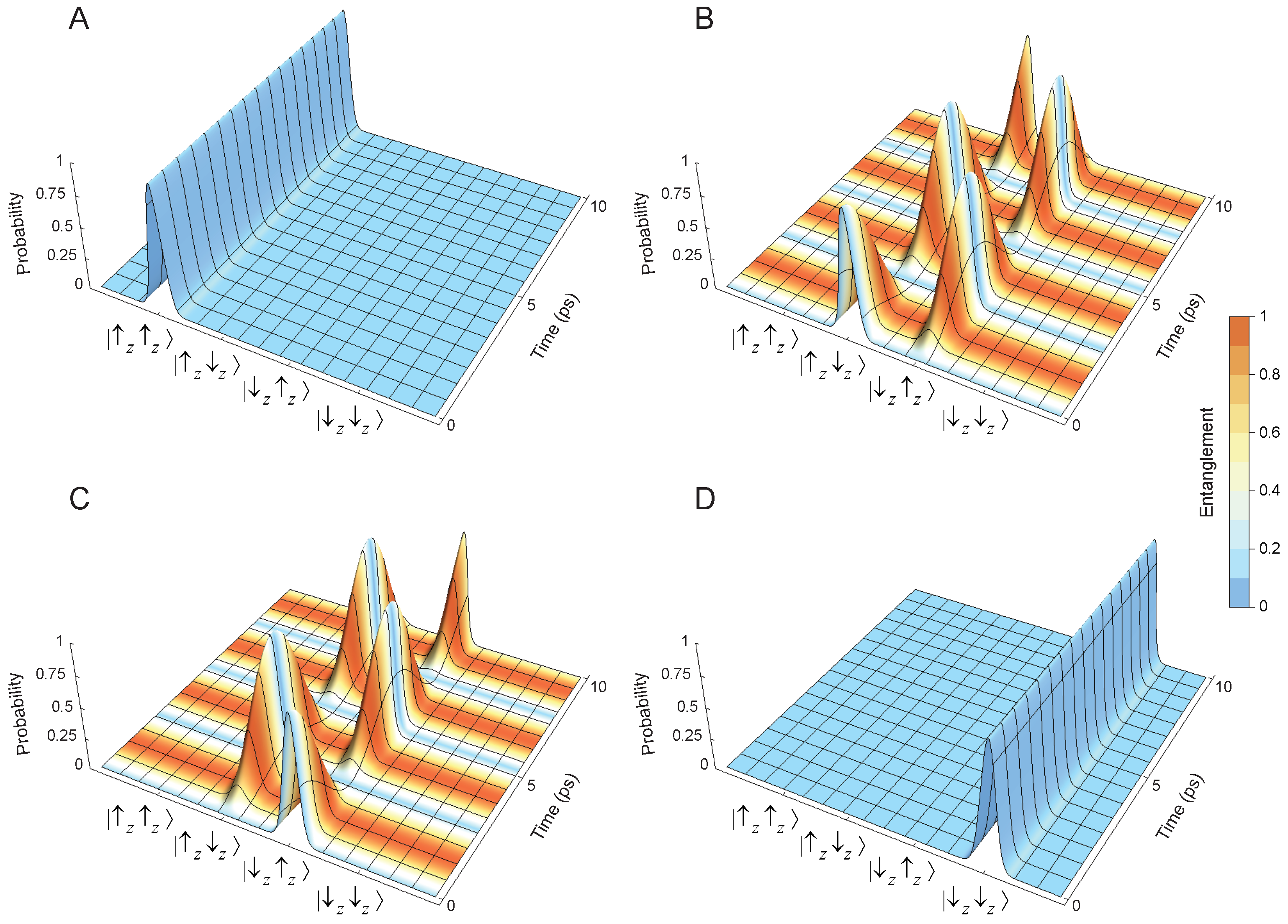
In the presence of non-zero interaction Hamiltonian, the quantum dynamics of the composite state vector $|\mathsf{\Psi }(t)\rangle$ is able to undergo cycles of quantum entanglement and disentanglement depending on the choice of the initial state vector $|\mathsf{\Psi }(0)\rangle$. From Equations (83)–(86) describing the time evolution of the quantum probabilities, it can be concluded that if the initial state is $|\mathsf{\Psi }\left(0\right)\rangle ={|\uparrow }_z{\uparrow }_z\rangle$ then its associated observable represented by the expectation value of the projection operator $\widehat{\mathcal{P}}\left({\uparrow }_z{\uparrow }_z\right)={|\uparrow }_z{\uparrow }_z{\rangle \langle \uparrow }_z{\uparrow }_z|$ does not evolve but stays constant $\langle \mathsf{\Psi }\left(t\right)|\widehat{\mathcal{P}}\left({\uparrow }_z{\uparrow }_z\right)|\mathsf{\Psi }\left(t\right)\rangle =1$ at all times (Figure 2A). From (45), it can be seen that the quantum evolution of the quantum state is to rotate in the Hilbert space with a pure phase $e^{-ı{\omega }_{1}t}{|\uparrow }_z{\uparrow }_z\rangle$, which leaves the state separable at all times. It is worth emphasizing that the quantum state evolves, whereas the expectation value of the projection operator does not. This illustrates clearly the fact that in the quantum world what is observed is not what exists, namely, the quantum observables (represented by matrix operators) are not quantum states (represented by state vectors). Similarly, if the initial state is $|\mathsf{\Psi }\left(0\right)\rangle ={|\downarrow }_z{\downarrow }_z\rangle$ then its associated observable represented by the expectation value of the projection operator $\widehat{\mathcal{P}}\left({\downarrow }_z{\downarrow }_z\right)={|\downarrow }_z{\downarrow }_z{\rangle \langle \downarrow }_z{\downarrow }_z|$ does not evolve but stays constant $\langle \mathsf{\Psi }\left(t\right)|\widehat{\mathcal{P}}\left({\downarrow }_z{\downarrow }_z\right)|\mathsf{\Psi }\left(t\right)\rangle =1$ at all times. Again, the quantum evolution of the quantum state is to rotate in the Hilbert space with a pure phase $e^{-ı{\omega }_{4}t}{|\downarrow }_z{\downarrow }_z\rangle$ thereby leaving the state separable at all times (Figure 2D). Interesting quantum dynamics results when the initial state is $|\mathsf{\Psi }\left(0\right)\rangle ={|\uparrow }_z{\downarrow }_z\rangle$ or $|\mathsf{\Psi }\left(0\right)\rangle ={|\downarrow }_z{\uparrow }_z\rangle$. In such cases, the expectation values of the corresponding projection operators evolve in time and there are observable quantum interference effects that can be recorded by external measurement devices (Figure 2B,C). Furthermore, the state repeatedly gets entangled, when $\mathrm{Prob}\left({\uparrow }_z{\downarrow }_z\right)=\mathrm{Prob}\left({\downarrow }_z{\uparrow }_z\right)=\frac{1}{2}$, followed by disentanglement, when one of the latter two probabilities becomes unit and the other becomes zero. Thus, initially separable composite quantum states are able to get quantum entangled if the interaction Hamiltonian is non-zero.

In order to see what the role of the interaction Hamiltonian is, we can turn it off by setting it to zero. In the absence of interaction Hamiltonian, the quantum dynamics of the composite state vector $|\mathsf{\Psi }(t)\rangle$ is no longer able to undergo cycles of quantum entanglement and disentanglement (Figure 3). Instead, the initially separable quantum states $|\mathsf{\Psi }(0)\rangle$ remain separable at all times, as indicated by the zero normalized entanglement number, $e\left(\mathsf{\Psi }\right)/e{\left(\mathsf{\Psi }\right)}_{max}=0$. Furthermore, the expectation values stay constant 1 for the particular projector $\widehat{\mathcal{P}}\left({\uparrow }_z{\uparrow }_z\right)$, $\widehat{\mathcal{P}}\left({\uparrow }_z{\downarrow }_z\right)$, $\widehat{\mathcal{P}}\left({\downarrow }_z{\uparrow }_z\right)$ or $\widehat{\mathcal{P}}\left({\downarrow }_z{\downarrow }_z\right)$ that corresponds to the initial state $|\mathsf{\Psi }(0)\rangle$ (Figure 3A–D). Thus, the presence of non-zero interaction Hamiltonian is essential for the generation of quantum entanglement starting from an initially separable quantum state $|\mathsf{\Psi }(0)\rangle$.

By pairwise comparison of the computer plots performed with or without non-zero interaction Hamiltonian, it can be seen that there is a difference in the quantum dynamics if the initial state is ${|\uparrow }_z{\downarrow }_z\rangle$ as shown in Figure 2B and Figure 3B, or ${|\downarrow }_z{\uparrow }_z\rangle$ as shown in Figure 2C and Figure 3C. Yet, there is no difference in the quantum dynamics if the initial state is ${|\uparrow }_z{\uparrow }_z\rangle$ as shown Figure 2A and Figure 3A, or ${|\downarrow }_z{\downarrow }_z\rangle$ as shown in Figure 2D and Figure 3D. The explanation for these findings is that the quantum dynamics for spin $zz$ states is governed by the presence of non-zero off-diagonal elements in the interaction Hamiltonian in the $zz$ basis

$${\widehat{H}}_{\mathrm{int}}=\frac{{\hslash }^2}{4}\xi \left(\begin{array}{cccc}1& 0& 0& 0\\ 0& -1& 2& 0\\ 0& 2& -1& 0\\ 0& 0& 0& 1\end{array}\right).$$

(92)

The first and fourth rows, which correspond respectively to the states ${|\uparrow }_z{\uparrow }_z\rangle$ and ${|\downarrow }_z{\downarrow }_z\rangle$, already contain off-diagonal zeroes, hence the zeroing of the interaction Hamiltonian does not change anything. On the other hand, only the second and third rows, which correspond respectively to the states ${|\uparrow }_z{\downarrow }_z\rangle$ and ${|\downarrow }_z{\uparrow }_z\rangle$ contain non-zero off-diagonal elements (coherences). Zeroing of the interaction Hamiltonian removes those non-zero off-diagonal elements, which in turn prevents the two qubits from interacting with each other and getting quantum entangled.

7.2. Complementary Observables in Spin $xx$ Basis

The non-commutativity of quantum operators results in incompatibility of the corresponding observables, which cannot be measured with a single experimental setting. Instead, measurements of incompatible quantum observables require different mutually incompatible settings of the employed experimental apparatus.

Suppose that we want to measure the two spins in x-direction. We need to consider the relations

$$\begin{array}{cc}\hfill {|\uparrow }_z\rangle & =\frac{1}{\sqrt{2}}\left({|\uparrow }_x{\rangle +|\downarrow }_x\rangle \right)\hfill \end{array}$$

(93)

$$\begin{array}{cc}\hfill {|\downarrow }_z\rangle & =\frac{1}{\sqrt{2}}\left({|\uparrow }_x{\rangle -|\downarrow }_x\rangle \right).\hfill \end{array}$$

(94)

Multiplying out the tensor products

$$\begin{array}{cc}\hfill {|\uparrow }_z{\uparrow }_z\rangle & =\frac{1}{2}\left({|\uparrow }_x{\rangle +|\downarrow }_x\rangle \right)\left({|\uparrow }_x{\rangle +|\downarrow }_x\rangle \right)\hfill \end{array}$$

(95)

$$\begin{array}{cc}\hfill {|\uparrow }_z{\downarrow }_z\rangle & =\frac{1}{2}\left({|\uparrow }_x{\rangle +|\downarrow }_x\rangle \right)\left({|\uparrow }_x{\rangle -|\downarrow }_x\rangle \right)\hfill \end{array}$$

(96)

$$\begin{array}{cc}\hfill {|\downarrow }_z{\uparrow }_z\rangle & =\frac{1}{2}\left({|\uparrow }_x{\rangle -|\downarrow }_x\rangle \right)\left({|\uparrow }_x{\rangle +|\downarrow }_x\rangle \right)\hfill \end{array}$$

(97)

$$\begin{array}{cc}\hfill {|\downarrow }_z{\downarrow }_z\rangle & =\frac{1}{2}\left({|\uparrow }_x{\rangle -|\downarrow }_x\rangle \right)\left({|\uparrow }_x{\rangle -|\downarrow }_x\rangle \right),\hfill \end{array}$$

(98)

we obtain

$$\begin{array}{cc}\hfill {|\uparrow }_z{\uparrow }_z\rangle & =\frac{1}{2}\left({|\uparrow }_x{\uparrow }_x{\rangle +|\uparrow }_x{\downarrow }_x{\rangle +|\downarrow }_x{\uparrow }_x{\rangle +|\downarrow }_x{\downarrow }_x\rangle \right)\hfill \end{array}$$

(99)

$$\begin{array}{cc}\hfill {|\uparrow }_z{\downarrow }_z\rangle & =\frac{1}{2}\left({|\uparrow }_x{\uparrow }_x{\rangle -|\uparrow }_x{\downarrow }_x{\rangle +|\downarrow }_x{\uparrow }_x{\rangle -|\downarrow }_x{\downarrow }_x\rangle \right)\hfill \end{array}$$

(100)

$$\begin{array}{cc}\hfill {|\downarrow }_z{\uparrow }_z\rangle & =\frac{1}{2}\left({|\uparrow }_x{\uparrow }_x{\rangle +|\uparrow }_x{\downarrow }_x{\rangle -|\downarrow }_x{\uparrow }_x{\rangle -|\downarrow }_x{\downarrow }_x\rangle \right)\hfill \end{array}$$

(101)

$$\begin{array}{cc}\hfill {|\downarrow }_z{\downarrow }_z\rangle & =\frac{1}{2}\left({|\uparrow }_x{\uparrow }_x{\rangle -|\uparrow }_x{\downarrow }_x{\rangle -|\downarrow }_x{\uparrow }_x{\rangle +|\downarrow }_x{\downarrow }_x\rangle \right).\hfill \end{array}$$

(102)

Upon setting $C_{\pm }=C_2\pm C_1$ and substitution of (99)–(102) into (45), we obtain the quantum state in spin $xx$ basis

$$\begin{array}{cc}\hfill |\mathsf{\Psi }(t)\rangle & =\frac{1}{2}\left[{\alpha }_1\left(0\right)e^{-ı{\omega }_{1}t}+C_{-}{\alpha }_2\left(0\right)e^{-ı{\omega }_{2}t}+C_{+}{\alpha }_3\left(0\right)e^{-ı{\omega }_{3}t}+{\alpha }_4\left(0\right)e^{-ı{\omega }_{4}t}\right]{|\uparrow }_x{\uparrow }_x\rangle \hfill \\ \hfill & +\frac{1}{2}\left[{\alpha }_1\left(0\right)e^{-ı{\omega }_{1}t}+C_{+}{\alpha }_2\left(0\right)e^{-ı{\omega }_{2}t}-C_{-}{\alpha }_3\left(0\right)e^{-ı{\omega }_{3}t}-{\alpha }_4\left(0\right)e^{-ı{\omega }_{4}t}\right]{|\uparrow }_x{\downarrow }_x\rangle \hfill \\ \hfill & +\frac{1}{2}\left[{\alpha }_1\left(0\right)e^{-ı{\omega }_{1}t}-C_{+}{\alpha }_2\left(0\right)e^{-ı{\omega }_{2}t}+C_{-}{\alpha }_3\left(0\right)e^{-ı{\omega }_{3}t}-{\alpha }_4\left(0\right)e^{-ı{\omega }_{4}t}\right]{|\downarrow }_x{\uparrow }_x\rangle \hfill \\ \hfill & +\frac{1}{2}\left[{\alpha }_1\left(0\right)e^{-ı{\omega }_{1}t}-C_{-}{\alpha }_2\left(0\right)e^{-ı{\omega }_{2}t}-C_{+}{\alpha }_3\left(0\right)e^{-ı{\omega }_{3}t}+{\alpha }_4\left(0\right)e^{-ı{\omega }_{4}t}\right]{|\downarrow }_x{\downarrow }_x\rangle .\hfill \end{array}$$

(103)

The probabilities of spin $xx$ observables are

$$\begin{array}{cc}\hfill \mathrm{Prob}\left({\uparrow }_x{\uparrow }_x\right)& =\frac{1}{4}{\left|{\alpha }_1\left(0\right)\right|}^2+\frac{1}{2}{C}_{-}\left|{\alpha }_1\left(0\right){\alpha }_2\left(0\right)\right|cos\left[\left({\omega }_1-{\omega }_2\right)t-{\phi }_1+{\phi }_2\right]\hfill \\ \hfill & +\frac{1}{2}{C}_{+}\left|{\alpha }_1\left(0\right){\alpha }_3\left(0\right)\right|cos\left[\left({\omega }_1-{\omega }_3\right)t-{\phi }_1+{\phi }_3\right]\hfill \\ \hfill & +\frac{1}{2}\left|{\alpha }_1\left(0\right){\alpha }_4\left(0\right)\right|cos\left[\left({\omega }_1-{\omega }_4\right)t-{\phi }_1+{\phi }_4\right]+\frac{1}{4}{C}_{-}^2{\left|{\alpha }_2\left(0\right)\right|}^2\hfill \\ \hfill & +\frac{1}{2}{C}_{+}{C}_{-}\left|{\alpha }_2\left(0\right){\alpha }_3\left(0\right)\right|cos\left[\left({\omega }_2-{\omega }_3\right)t-{\phi }_2+{\phi }_3\right]\hfill \\ \hfill & +\frac{1}{2}{C}_{-}\left|{\alpha }_2\left(0\right){\alpha }_4\left(0\right)\right|cos\left[\left({\omega }_2-{\omega }_4\right)t-{\phi }_2+{\phi }_4\right]+\frac{1}{4}{C}_{+}^2{\left|{\alpha }_3\left(0\right)\right|}^2\hfill \\ \hfill & +\frac{1}{2}{C}_{+}\left|{\alpha }_3\left(0\right){\alpha }_4\left(0\right)\right|cos\left[\left({\omega }_3-{\omega }_4\right)t-{\phi }_3+{\phi }_4\right]+\frac{1}{4}{\left|{\alpha }_4\left(0\right)\right|}^2\hfill \end{array}$$

(104)

$$\begin{array}{cc}\hfill \mathrm{Prob}\left({\uparrow }_x{\downarrow }_x\right)& =\frac{1}{4}{\left|{\alpha }_1\left(0\right)\right|}^2+\frac{1}{2}{C}_{+}\left|{\alpha }_1\left(0\right){\alpha }_2\left(0\right)\right|cos\left[\left({\omega }_1-{\omega }_2\right)t-{\phi }_1+{\phi }_2\right]\hfill \\ \hfill & -\frac{1}{2}{C}_{-}\left|{\alpha }_1\left(0\right){\alpha }_3\left(0\right)\right|cos\left[\left({\omega }_1-{\omega }_3\right)t-{\phi }_1+{\phi }_3\right]\hfill \\ \hfill & -\frac{1}{2}\left|{\alpha }_1\left(0\right){\alpha }_4\left(0\right)\right|cos\left[\left({\omega }_1-{\omega }_4\right)t-{\phi }_1+{\phi }_4\right]+\frac{1}{4}{C}_{+}^2{\left|{\alpha }_2\left(0\right)\right|}^2\hfill \\ \hfill & -\frac{1}{2}{C}_{+}{C}_{-}\left|{\alpha }_2\left(0\right){\alpha }_3\left(0\right)\right|cos\left[\left({\omega }_2-{\omega }_3\right)t-{\phi }_2+{\phi }_3\right]\hfill \\ \hfill & -\frac{1}{2}{C}_{+}\left|{\alpha }_2\left(0\right){\alpha }_4\left(0\right)\right|cos\left[\left({\omega }_2-{\omega }_4\right)t-{\phi }_2+{\phi }_4\right]+\frac{1}{4}{C}_{-}^2{\left|{\alpha }_3\left(0\right)\right|}^2\hfill \\ \hfill & +\frac{1}{2}{C}_{-}\left|{\alpha }_3\left(0\right){\alpha }_4\left(0\right)\right|cos\left[\left({\omega }_3-{\omega }_4\right)t-{\phi }_3+{\phi }_4\right]+\frac{1}{4}{\left|{\alpha }_4\left(0\right)\right|}^2\hfill \end{array}$$

(105)

$$\begin{array}{cc}\hfill \mathrm{Prob}\left({\downarrow }_x{\uparrow }_x\right)& =\frac{1}{4}{\left|{\alpha }_1\left(0\right)\right|}^2-\frac{1}{2}{C}_{+}\left|{\alpha }_1\left(0\right){\alpha }_2\left(0\right)\right|cos\left[\left({\omega }_1-{\omega }_2\right)t-{\phi }_1+{\phi }_2\right]\hfill \\ \hfill & +\frac{1}{2}{C}_{-}\left|{\alpha }_1\left(0\right){\alpha }_3\left(0\right)\right|cos\left[\left({\omega }_1-{\omega }_3\right)t-{\phi }_1+{\phi }_3\right]\hfill \\ \hfill & -\frac{1}{2}\left|{\alpha }_1\left(0\right){\alpha }_4\left(0\right)\right|cos\left[\left({\omega }_1-{\omega }_4\right)t-{\phi }_1+{\phi }_4\right]+\frac{1}{4}{C}_{+}^2{\left|{\alpha }_2\left(0\right)\right|}^2\hfill \\ \hfill & -\frac{1}{2}{C}_{+}{C}_{-}\left|{\alpha }_2\left(0\right){\alpha }_3\left(0\right)\right|cos\left[\left({\omega }_2-{\omega }_3\right)t-{\phi }_2+{\phi }_3\right]\hfill \\ \hfill & +\frac{1}{2}{C}_{+}\left|{\alpha }_2\left(0\right){\alpha }_4\left(0\right)\right|cos\left[\left({\omega }_2-{\omega }_4\right)t-{\phi }_2+{\phi }_4\right]+\frac{1}{4}{C}_{-}^2{\left|{\alpha }_3\left(0\right)\right|}^2\hfill \\ \hfill & -\frac{1}{2}{C}_{-}\left|{\alpha }_3\left(0\right){\alpha }_4\left(0\right)\right|cos\left[\left({\omega }_3-{\omega }_4\right)t-{\phi }_3+{\phi }_4\right]+\frac{1}{4}{\left|{\alpha }_4\left(0\right)\right|}^2\hfill \end{array}$$

(106)

$$\begin{array}{cc}\hfill \mathrm{Prob}\left({\downarrow }_x{\downarrow }_x\right)& =\frac{1}{4}{\left|{\alpha }_1\left(0\right)\right|}^2-\frac{1}{2}{C}_{-}\left|{\alpha }_1\left(0\right){\alpha }_2\left(0\right)\right|cos\left[\left({\omega }_1-{\omega }_2\right)t-{\phi }_1+{\phi }_2\right]\hfill \\ \hfill & -\frac{1}{2}{C}_{+}\left|{\alpha }_1\left(0\right){\alpha }_3\left(0\right)\right|cos\left[\left({\omega }_1-{\omega }_3\right)t-{\phi }_1+{\phi }_3\right]\hfill \\ \hfill & +\frac{1}{2}\left|{\alpha }_1\left(0\right){\alpha }_4\left(0\right)\right|cos\left[\left({\omega }_1-{\omega }_4\right)t-{\phi }_1+{\phi }_4\right]+\frac{1}{4}{C}_{-}^2{\left|{\alpha }_2\left(0\right)\right|}^2\hfill \\ \hfill & +\frac{1}{2}{C}_{+}{C}_{-}\left|{\alpha }_2\left(0\right){\alpha }_3\left(0\right)\right|cos\left[\left({\omega }_2-{\omega }_3\right)t-{\phi }_2+{\phi }_3\right]\hfill \\ \hfill & -\frac{1}{2}{C}_{-}\left|{\alpha }_2\left(0\right){\alpha }_4\left(0\right)\right|cos\left[\left({\omega }_2-{\omega }_4\right)t-{\phi }_2+{\phi }_4\right]+\frac{1}{4}{C}_{+}^2{\left|{\alpha }_3\left(0\right)\right|}^2\hfill \\ \hfill & -\frac{1}{2}{C}_{+}\left|{\alpha }_3\left(0\right){\alpha }_4\left(0\right)\right|cos\left[\left({\omega }_3-{\omega }_4\right)t-{\phi }_3+{\phi }_4\right]+\frac{1}{4}{\left|{\alpha }_4\left(0\right)\right|}^2.\hfill \end{array}$$

(107)

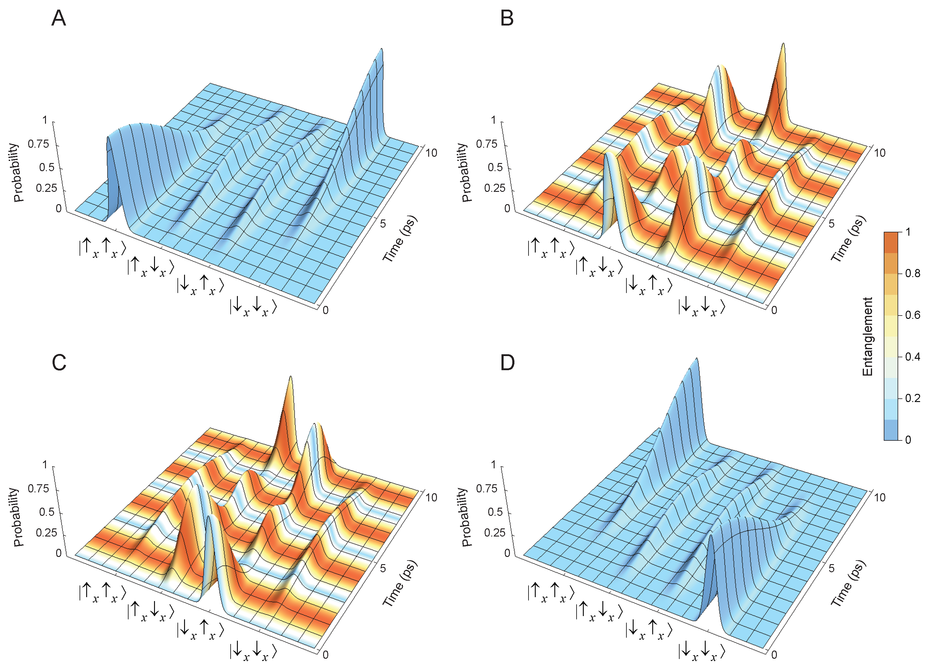
Computer simulations confirm again that in the presence of non-zero interaction Hamiltonian the quantum dynamics of the composite state vector $|\mathsf{\Psi }(t)\rangle$ is able to undergo cycles of quantum entanglement and disentanglement depending on the choice of the initial state vector $|\mathsf{\Psi }(0)\rangle$ (Figure 4). When, the initial state is $|\mathsf{\Psi }\left(0\right)\rangle ={|\uparrow }_x{\uparrow }_x\rangle$ (Figure 4A) or $|\mathsf{\Psi }\left(0\right)\rangle ={|\downarrow }_x{\downarrow }_x\rangle$ (Figure 4D), the quantum dynamics leaves the state $|\mathsf{\Psi }(t)\rangle$ separable at all times, as indicated by the zero normalized entanglement number, $e\left(\mathsf{\Psi }\right)/e{\left(\mathsf{\Psi }\right)}_{max}=0$. However, in these cases each qubit manifests its own quantum interference pattern, which is independent on the interference pattern manifested by the other qubit. This, reveals the importance of the internal Hamiltonians to generate quantum interference patterns only within the reduced subspaces of the component subsystems. When, the initial state is $|\mathsf{\Psi }\left(0\right)\rangle ={|\uparrow }_x{\downarrow }_x\rangle$ (Figure 4B) or $|\mathsf{\Psi }\left(0\right)\rangle ={|\downarrow }_x{\uparrow }_x\rangle$ (Figure 4C), the quantum dynamics of the state $|\mathsf{\Psi }(t)\rangle$ undergoes cycles of quantum entanglement and disentanglement. In the presence of quantum entanglement, the quantum interference patterns manifested by the two qubits become correlated, which can be appreciated by comparison with the case when the interaction Hamiltonian is turned off.

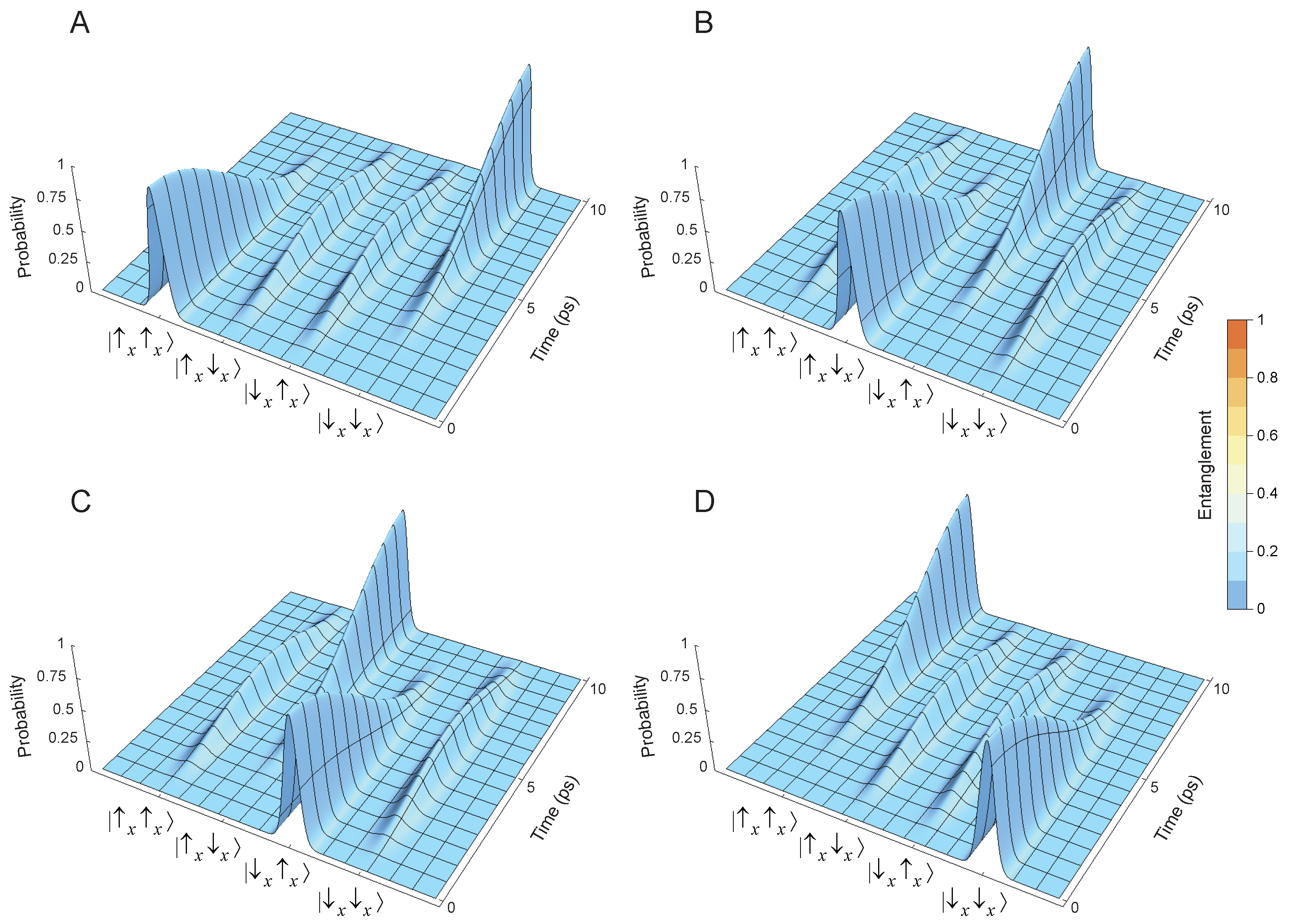
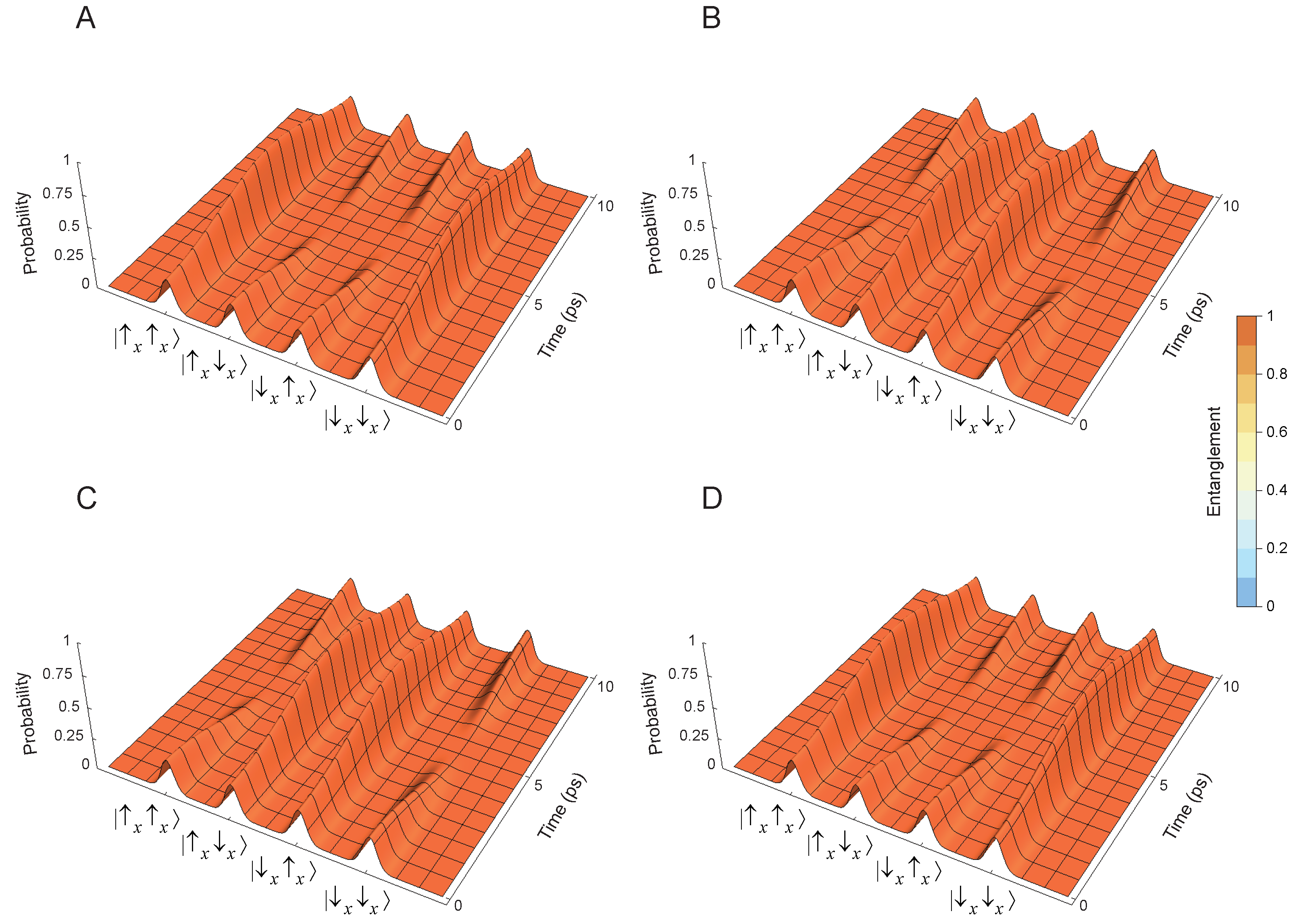
In the absence of interaction Hamiltonian (Figure 5), the quantum dynamics can no longer generate quantum entanglement from initially separable composite quantum state $|\mathsf{\Psi }(0)\rangle$. For all four initial quantum states, the quantum dynamics leaves the state $|\mathsf{\Psi }(t)\rangle$ separable at all times. When the initial state is $|\mathsf{\Psi }\left(0\right)\rangle ={|\uparrow }_x{\uparrow }_x\rangle$ (Figure 5A) or $|\mathsf{\Psi }\left(0\right)\rangle ={|\downarrow }_x{\downarrow }_x\rangle$ (Figure 5D), the expectation values for the projectors $\widehat{\mathcal{P}}\left({\uparrow }_x{\uparrow }_x\right)$, $\widehat{\mathcal{P}}\left({\uparrow }_x{\downarrow }_x\right)$, $\widehat{\mathcal{P}}\left({\downarrow }_x{\uparrow }_x\right)$ and $\widehat{\mathcal{P}}\left({\downarrow }_x{\downarrow }_x\right)$ remain the same as in the corresponding cases with non-zero interaction Hamiltonian (Figure 4A,D). However, when the initial state is $|\mathsf{\Psi }\left(0\right)\rangle ={|\uparrow }_x{\downarrow }_x\rangle$ (Figure 5B) or $|\mathsf{\Psi }\left(0\right)\rangle ={|\downarrow }_x{\uparrow }_x\rangle$ (Figure 5C), the expectation values for the projectors $\widehat{\mathcal{P}}\left({\uparrow }_x{\uparrow }_x\right)$, $\widehat{\mathcal{P}}\left({\uparrow }_x{\downarrow }_x\right)$, $\widehat{\mathcal{P}}\left({\downarrow }_x{\uparrow }_x\right)$ and $\widehat{\mathcal{P}}\left({\downarrow }_x{\downarrow }_x\right)$ differ from those shown in the corresponding cases with non-zero interaction Hamiltonian (Figure 4B,C). The explanation of these findings is based on the presence or absence of non-zero off-diagonal elements (coherences) in the interaction Hamiltonian when expressed in the spin $xx$ basis, analogously to the explanation that was already given for the spin $zz$ observables. In fact, the matrix form (92) of the interaction Hamiltonian is preserved exactly the same during the conversion from spin $zz$ basis to spin $xx$ basis. Noteworthy, the internal Hamiltonians ${\widehat{H}}_A$ and ${\widehat{H}}_B$ do change their matrix form during the conversion from spin $zz$ basis to spin $xx$ basis, which in turn explains why the expectation values of spin $xx$ or spin $zz$ observables for initial states where both spins start aligned in the same direction, either display quantum interference patterns (Figure 5A,D) or stay constant (Figure 3A,D), respectively.

8. Quantum Dynamics of Initial Quantum Entangled States

The importance of non-zero interaction Hamiltonian for entangling two qubits starting from an initially separable quantum state, goes in the other direction as well. In other words, non-zero interaction Hamiltonian is required to disentangle two qubits starting from an initially entangled quantum state. For illustration, consider the following four maximally entangled initial states $|\mathsf{\Psi }(0)\rangle$ given by

$$\begin{array}{cc}\hfill \frac{1}{\sqrt{2}}\left({|\uparrow }_z{\uparrow }_x{\rangle +|\downarrow }_z{\downarrow }_x\rangle \right)& =\frac{1}{2}\left(|E_1\rangle +C_{-}|E_2\rangle +C_{+}|E_3\rangle -|E_4\rangle \right)\hfill \end{array}$$

(108)

$$\begin{array}{cc}\hfill \frac{1}{\sqrt{2}}\left({|\uparrow }_z{\downarrow }_x{\rangle +|\downarrow }_z{\uparrow }_x\rangle \right)& =\frac{1}{2}\left(|E_1\rangle +C_{+}|E_2\rangle -C_{-}|E_3\rangle +|E_4\rangle \right)\hfill \end{array}$$

(109)

$$\begin{array}{cc}\hfill \frac{1}{\sqrt{2}}\left({|\uparrow }_z{\uparrow }_x{\rangle -|\downarrow }_z{\downarrow }_x\rangle \right)& =\frac{1}{2}\left(|E_1\rangle -C_{+}|E_2\rangle +C_{-}|E_3\rangle +|E_4\rangle \right)\hfill \end{array}$$

(110)

$$\begin{array}{cc}\hfill \frac{1}{\sqrt{2}}\left({|\uparrow }_z{\downarrow }_x{\rangle -|\downarrow }_z{\uparrow }_x\rangle \right)& =\frac{1}{2}\left(|E_1\rangle -C_{-}|E_2\rangle -C_{+}|E_3\rangle -|E_4\rangle \right)\hfill \end{array}$$

(111)

and suppose that we measure the expectation values of the projectors $\widehat{\mathcal{P}}\left({\uparrow }_x{\uparrow }_x\right)$, $\widehat{\mathcal{P}}\left({\uparrow }_x{\downarrow }_x\right)$, $\widehat{\mathcal{P}}\left({\downarrow }_x{\uparrow }_x\right)$ and $\widehat{\mathcal{P}}\left({\downarrow }_x{\downarrow }_x\right)$. When the initial state $|\mathsf{\Psi }(0)\rangle$ is $\frac{1}{\sqrt{2}}\left({|\uparrow }_z{\uparrow }_x{\rangle +|\downarrow }_z{\downarrow }_x\rangle \right)$ (Figure 6A) or $\frac{1}{\sqrt{2}}\left({|\uparrow }_z{\downarrow }_x{\rangle -|\downarrow }_z{\uparrow }_x\rangle \right)$ (Figure 6D), the state $|\mathsf{\Psi }(t)\rangle$ remains maximally entangled at all times even though the spin $xx$ observables undergo dynamics that manifests quantum interference patterns. However, when the initial state $|\mathsf{\Psi }(0)\rangle$ is $\frac{1}{\sqrt{2}}\left({|\uparrow }_z{\downarrow }_x{\rangle +|\downarrow }_z{\uparrow }_x\rangle \right)$ (Figure 6B) or $\frac{1}{\sqrt{2}}\left({|\uparrow }_z{\uparrow }_x{\rangle -|\downarrow }_z{\downarrow }_x\rangle \right)$ (Figure 6C), the state $|\mathsf{\Psi }(t)\rangle$ undergoes cycles of disentanglement and entanglement. The time points at which the composite quantum state $|\mathsf{\Psi }(t)\rangle$ becomes separable coincide with unit quantum probability creating a peak at one of the two states ${|\uparrow }_x{\downarrow }_x\rangle$ or ${|\downarrow }_x{\uparrow }_x\rangle$, while all other orthogonal basis states remain empty with zero quantum probability.

In the case when the interaction Hamiltonian is turned off, all four maximally entangled initial quantum states $\frac{1}{\sqrt{2}}\left({|\uparrow }_z{\uparrow }_x{\rangle +|\downarrow }_z{\downarrow }_x\rangle \right)$ (Figure 7A), $\frac{1}{\sqrt{2}}\left({|\uparrow }_z{\downarrow }_x{\rangle +|\downarrow }_z{\uparrow }_x\rangle \right)$ (Figure 7B), $\frac{1}{\sqrt{2}}\left({|\uparrow }_z{\uparrow }_x{\rangle -|\downarrow }_z{\downarrow }_x\rangle \right)$ (Figure 7C) and $\frac{1}{\sqrt{2}}\left({|\uparrow }_z{\downarrow }_x{\rangle -|\downarrow }_z{\uparrow }_x\rangle \right)$ (Figure 7D) undergo quantum dynamics that leaves the composite state $|\mathsf{\Psi }(t)\rangle$ maximally entangled at all times. Now, we are ready to prove a general theorem according to which quantum dynamics resulting only from internal Hamiltonians is unable to change the amount of quantum entanglement that is already possessed by the initial quantum state.

Theorem 4.

Unitary quantum dynamics resulting from the Schrödinger equation that is only due to internal Hamiltonians is unable to change the amount of quantum entanglement that is already present in the initial composite quantum state $|\mathsf{\Psi }(0)\rangle$.

Proof. 

Without loss of generality, suppose that we have a composite system of two qubits governed by the Hamiltonian

$$\widehat{H}={\widehat{H}}_A\otimes {\widehat{I}}_B+{\widehat{I}}_A\otimes {\widehat{H}}_B.$$

(112)

Express the initial quantum state in Schmidt basis

$$|\mathsf{\Psi }\left(0\right)\rangle ={\lambda }_1{|\uparrow }_A{\rangle |\uparrow }_B\rangle +{\lambda }_2{|\downarrow }_A{\rangle |\downarrow }_B\rangle ,$$

(113)

where the basis vectors are orthogonal

$${\langle \downarrow }_A{|\uparrow }_A{\rangle =\langle \downarrow }_B{|\uparrow }_B\rangle =0.$$

(114)

Solving the Schrödinger equation gives the composite quantum state at any time point t using the matrix exponential of the Hamiltonian

$$|\mathsf{\Psi }\left(t\right)\rangle =e^{-\frac{ı}{\hslash }\left({\widehat{H}}_A\otimes {\widehat{I}}_B+{\widehat{I}}_A\otimes {\widehat{H}}_B\right)t}|\mathsf{\Psi }\left(0\right)\rangle .$$

(115)

Using the commutativity of ${\widehat{H}}_A\otimes {\widehat{I}}_B$ and ${\widehat{I}}_A\otimes {\widehat{H}}_B$, namely, $\left[{\widehat{H}}_A\otimes {\widehat{I}}_B,{\widehat{I}}_A\otimes {\widehat{H}}_B\right]=0$, we can apply a special case of the Baker–Campbell–Hausdorff formula [75,76,77,78]

$$e^{-\frac{ı}{\hslash }\left({\widehat{H}}_A\otimes {\widehat{I}}_B+{\widehat{I}}_A\otimes {\widehat{H}}_B+\frac{1}{2}\left[{\widehat{H}}_A\otimes {\widehat{I}}_B,{\widehat{I}}_A\otimes {\widehat{H}}_B\right]\right)t}=e^{-\frac{ı}{\hslash }\left({\widehat{H}}_A\otimes {\widehat{I}}_B\right)t}{e}^{-\frac{ı}{\hslash }\left({\widehat{I}}_A\otimes {\widehat{H}}_B\right)t}.$$

(116)

Using the power series definition of the matrix exponential, we have

$$|\mathsf{\Psi }\left(t\right)\rangle =\sum _{k=0}^{\infty }\frac{1}{k!}{\left[-\frac{ı}{\hslash }\left({\widehat{H}}_A\otimes {\widehat{I}}_B\right)t\right]}^k\sum _{n=0}^{\infty }\frac{1}{n!}{\left[-\frac{ı}{\hslash }\left({\widehat{I}}_A\otimes {\widehat{H}}_B\right)t\right]}^n|\mathsf{\Psi }\left(0\right)\rangle .$$

(117)

Taking into account that powers of the identity operator are also identity, we obtain

$$|\mathsf{\Psi }\left(t\right)\rangle =\left(e^{-\frac{ı}{\hslash }{\widehat{H}}_{A}t}\otimes {\widehat{I}}_B\right)\left({\widehat{I}}_A\otimes e^{-\frac{ı}{\hslash }{\widehat{H}}_{B}t}\right)|\mathsf{\Psi }\left(0\right)\rangle =e^{-\frac{ı}{\hslash }{\widehat{H}}_{A}t}\otimes e^{-\frac{ı}{\hslash }{\widehat{H}}_{B}t}|\mathsf{\Psi }\left(0\right)\rangle .$$

(118)

Further substitution of the initial quantum state in Schmidt basis followed by distribution of the time evolution operators gives

$$|\mathsf{\Psi }\left(t\right)\rangle ={\lambda }_1{e}^{-\frac{ı}{\hslash }{\widehat{H}}_{A}t}{|\uparrow }_A\rangle \otimes e^{-\frac{ı}{\hslash }{\widehat{H}}_{B}t}{|\uparrow }_B\rangle +{\lambda }_2{e}^{-\frac{ı}{\hslash }{\widehat{H}}_{A}t}{|\downarrow }_A\rangle \otimes e^{-\frac{ı}{\hslash }{\widehat{H}}_{B}t}{|\downarrow }_B\rangle .$$

(119)

Because both internal time evolution operators $e^{-\frac{ı}{\hslash }{\widehat{H}}_{A}t}$ and $e^{-\frac{ı}{\hslash }{\widehat{H}}_{B}t}$ are unitary, they preserve inner products

$$\begin{array}{cc}\hfill \langle {\downarrow }_A\left(t\right)|{\uparrow }_A\left(t\right)\rangle & ={\langle \downarrow }_A|e^{\frac{ı}{\hslash }{\widehat{H}}_{A}t}{e}^{-\frac{ı}{\hslash }{\widehat{H}}_{A}t}{|\uparrow }_A{\rangle =\langle \downarrow }_A{|1|\uparrow }_A\rangle =0\hfill \end{array}$$

(120)

$$\begin{array}{cc}\hfill \langle {\downarrow }_B\left(t\right)|{\uparrow }_B\left(t\right)\rangle & ={\langle \downarrow }_B|e^{\frac{ı}{\hslash }{\widehat{H}}_{B}t}{e}^{-\frac{ı}{\hslash }{\widehat{H}}_{B}t}{|\uparrow }_B{\rangle =\langle \downarrow }_B{|1|\uparrow }_B\rangle =0.\hfill \end{array}$$

(121)

This implies that the time evolved composite state decomposed in Schmidt basis is

$$|\mathsf{\Psi }\left(t\right)\rangle ={\lambda }_1{|\uparrow }_A{\left(t\right)\rangle |\uparrow }_B\left(t\right)\rangle +{\lambda }_2{|\downarrow }_A{\left(t\right)\rangle |\downarrow }_B\left(t\right)\rangle ,$$

(122)

which has exactly the same Schmidt coefficients as $|\mathsf{\Psi }(0)\rangle$. The amount of quantum entanglement measured by the entanglement number $e\left(\mathsf{\Psi }\right)$ is only a function of the two Schmidt coefficients ${\lambda }_1$ and ${\lambda }_2$. Therefore, during quantum dynamics that is only due to internal Hamiltonians, the entanglement number stays constant, $e\left[\mathsf{\Psi }\left(0\right)\right]=e\left[\mathsf{\Psi }\left(t\right)\right]$. Note that we did not resort anywhere in the proof to the fact that we have only two component systems, or that the individual Hilbert spaces have only two complex dimensions. Hence, the presented proof straightforwardly generalizes to multipartite systems with an arbitrary number of dimensions of the individual Hilbert spaces. □

9. Quantum Coherence Cannot Bind Conscious Experiences

Having explored the precise meaning of various quantum information-theoretic concepts, we are ready to apply quantum information theory to a specific problem of consciousness, namely, the problem of binding of conscious experiences.

Definition 7.

(Single mind) Awake healthy humans experience an integrated mental picture consisting of visual, auditory, gustatory, olfactory, and sensorimotor perceptions. Being a single mind can be understood introspectively as the total content of all conscious experiences that you have at a single time instant. Single minds are conscious [8].

Definition 8.

(Collection of minds) Being within a collection of minds can be understood through contemplation of what it is like to be a participant in a conversation with another human. When you talk with a friend, you may only guess what it is like to be inside your friend’s mind, but you do not have direct access to your friend’s conscious experiences. Thus, you and your friend are two separate minds. Taken together, you and your friend, form a collection of minds. The collection of conscious minds is not conscious because it does not possess a single mind [8].

Some quantum mind advocates use the phrase quantum coherence as a magical buzzword that presumably explains the physical mechanism that binds your conscious experience, e.g., your visual experiences with your auditory experiences, into a single integrated conscious mind that is you. Unfortunately, this cannot be the case due to the intimate relationship between subsystem coherence and separability of the composite system as discussed in Section 5 and Section 6. The latter important point could be better appreciated by considering the following illuminating example.

Example 6.

(Alice and Bob have two separate minds) Take two people, Alice and Bob, each of which has an individual conscious mind. Let Alice have a mind defined by the pure (quantum coherent) state $|{\mathsf{\Psi }}_A\rangle$ and let Bob have a mind defined by the pure (quantum coherent) state $|{\mathsf{\Psi }}_B\rangle$. The quantum mechanical axioms for composition then imply that the composite system is also in a pure (quantum coherent) state $|{\mathsf{\Psi }}_{AB}\rangle =|{\mathsf{\Psi }}_A\rangle \otimes |{\mathsf{\Psi }}_B\rangle$. Obviously, if all pure (quantum coherent) states had a conscious mind, then $|{\mathsf{\Psi }}_{AB}\rangle$ would be paradoxically a global conscious mind as well [8]. In order to ban paradoxical occurrence of minds within other larger minds, quantum theory needs to postulate that factorizable non-entangled quantum states correspond to a collection of minds like Alice and Bob [23,24].

Theorem 5.

Quantum purity (colloquially referred to as “quantum coherence” in decoherence theory) is related to separability, non-interaction and lack of binding, rather than binding of conscious experiences.

Proof. 

Arrive at contradiction (i.e., occurrence of minds within other minds) by assuming the opposite (i.e., that quantum purity binds conscious experiences). In mathematical logic, arriving at contradiction implies that the assumed premise is false. □

Extremely cold temperatures in quantum technologies attempt to reduce the quantum interactions in order to ensure that the initial composite state of qubits is separable in the computational basis, and stays unaltered when no computational quantum gates are performed [79]. In other words, in order for human programmer to be able to extract any useful information from the quantum computation, the quantum computer should be isolated from interaction with its physical environment. However, we as conscious minds do not exist in a void isolated from interaction from the rest of the universe. On the contrary, we constantly receive sensory information from the surrounding world. What is more, we enjoy so greatly being aware of the surrounding world that total sensory deprivation of healthy human subjects in a dark room is experienced as a mental torture [80,81,82,83]. Furthermore, there is no external programmer who is supposed to extract useful information by observing the quantum state of our brain. Both of these points show that even the motivation behind quantum mind models insisting on preserving quantum coherence through putative isolation from the environment is faulty. Quantum dynamics of brain molecules occurs at picosecond timescale and rapid quantum entanglement due to quantum interactions could lead to extensive correlations between different quantum brain observables. Because composite quantum entangled states are much more complex than separable states, it is quite natural to expect that quantum entanglement due to quantum interactions is directly related to the complexity of conscious experiences, whereas quantum separability due to non-interaction of individually quantum coherent components is related to disbinding or splitting of conscious experiences into a collection of simpler, elementary minds [24].

Definition 9.

(Kolmogorov complexity) The complexity K of description of a given string of symbols S is the minimal number of classical information bits needed to describe the string S in some fixed universal description language [84,85].

Example 7.

(Condensation reduces complexity) Modeling consciousness in terms of condensation of multiple components in the same quantum state $|\psi \rangle \otimes |\psi \rangle \otimes \dots \otimes |\psi \rangle$ inside some kind of room temperature superconductor (as suggested in [86]) goes against the desirable link between complexity and richness of conscious experiences. Complexity of quantum states requires high level of entanglement as opposed to separability [87]. Consider a simple system of 3 qutrits whose Hilbert space $\mathcal{H}$ is $3\times 3\times 3=27$ dimensional. To specify a general quantum entangled state of these 3 qutrits, we will need 27 different complex quantum probability amplitudes

$$|\mathsf{\Psi }\rangle =\left(\begin{array}{c}{a}_1\\ a_2\\ ⋮\\ a_{27}\end{array}\right).$$

(123)

If we suppose that for the encoding of each $a_i$ (e.g., as a root of some polynomial equation) it takes K bits of information, for a general quantum entangled state we will need $27K$ bits.

If the state is factorizable, however, in the form

$$|\mathsf{\Psi }\rangle =\left(\begin{array}{c}{a}_1\\ a_2\\ a_3\end{array}\right)\otimes \left(\begin{array}{c}{a}_4\\ a_5\\ a_6\end{array}\right)\otimes \left(\begin{array}{c}{a}_7\\ a_8\\ a_9\end{array}\right),$$

(124)

then we will need only $3+3+3=9$ different complex quantum probability amplitudes to fully specify the separable tensor product state. Thus, for a general separable quantum state of 3 qutrits we will need $9K$ bits.

Finally, if all of the 3 qutrits are condensed in the same state

$$|\mathsf{\Psi }\rangle =\left(\begin{array}{c}{a}_1\\ a_2\\ a_3\end{array}\right)\otimes \left(\begin{array}{c}{a}_1\\ a_2\\ a_3\end{array}\right)\otimes \left(\begin{array}{c}{a}_1\\ a_2\\ a_3\end{array}\right),$$

(125)

then we will need only 3 different complex quantum probability amplitudes to fully specify the condensed state. The resulting complexity is only $3K$ bits. The problem with condensation is obvious, namely, the state becomes less and less complex, therefore conscious experiences will become poorer and poorer as the condensation progresses. In fact, the previous criticism with regard to quantum coherence and quantum separability also applies to condensation. In particular, quantum systems that are in a tensor product state are independent on each other and it makes no sense to claim that they have a single mind, on the contrary, there is a good reason to conclude that such quantum systems correspond to a collection of separate, independent minds.

10. Conclusions

Application of quantum information theory to studying neurophysiological processes is able to provide novel insights that are hard to anticipate from classical principles alone [8]. To amend the current lack of concise but rigorous introductions to quantum physics, we commenced this work with a brief description of the Hilbert space formalism of quantum mechanics and explained its physical meaning using a minimal quantum toy model. Then, employing the tools of quantum mechanics, we have determined the appropriate quantum dynamical timescale of cognitive processes and pinpointed the physical mechanism that binds conscious experiences within a single mind.

Our first main result is that the dynamic timescale of quantum processes, which supports consciousness, has to be constrained by the Planck–Einstein relation between energy and frequency. Because the typical energies driving biological processes are greater than the energy of the thermal noise, the resulting dynamics is fixed to picosecond timescale or faster, which is in the realm of quantum chemistry [88]. This requires rethinking of the role of classical neuronal electric spiking at millisecond timescale [89], not as generating elementary conscious events, but as a form of short term memory comprised of billions of almost identical picosecond conscious events [8]. Of course, the electric spike eventually fades away as the neuron repolarizes, which means that the ongoing stream of consciousness will forget the experiences that have triggered the spike unless another biological form of storing long term memories is used, such as changing the electric excitability of the neuronal membrane [90], strengthening of the activity of the stimulated synapses [91] or morphological reorganization of the axo-dendritic neuronal trees [92].

Our second main result is that the quantum interactions due to non-zero interaction Hamiltonian in the Schrödinger equation are responsible for dynamic changes in the amount of quantum entanglement, which leads to decoherence of the individual quantum subsystems along with their interaction. We also proved a rigorous quantum theorem according to which unitary quantum dynamics that is only due to internal Hamiltonians is unable to change the amount of quantum entanglement already present in the initial composite quantum state. This implies that turning off the interaction Hamiltonian will indeed preserve quantum coherence of individual component subsystems starting from an initially separable quantum state, however, the quantum probabilities for different physical observables measured on one of the subsystems will remain independent from those measured on the other subsystem, which in turn precludes any role of quantum coherence in cognitive binding of conscious experiences. In fact, decomposition of a composite quantum state into a tensor product of pure (quantum coherent) states is an indicator of splitting of different conscious experiences into a collection of individual conscious minds, whereas inseparability of a composite quantum entangled state is a possible indicator of binding of different conscious experiences into a single integrated conscious mind [8].

Studying the Schrödinger equation may appear intimidating, but it is a profitable investment that pays off with a high interest. The mathematical constraints that enter into the composition of a physically admissible Hamiltonian, together with the axioms that relate quantum states with the expectation values of quantum observables, are sufficient for the derivation of general quantum information-theoretic no-go theorems that hold for all physical processes including those that support consciousness [7,8]. These quantum theorems then could serve as theoretical tools to differentiate between plausible and implausible physical solutions of open problems in cognitive neuroscience.

References

- Duhem, P.M.M. The Aim and Structure of Physical Theory; Princeton University Press: Princeton, NJ, USA, 1954. [Google Scholar]
- Susskind, L.; Hrabovsky, G. The Theoretical Minimum: What You Need to Know to Start Doing Physics; Basic Books: New York, NY, USA, 2013. [Google Scholar]
- Landau, L.D.; Lifshitz, E.M. Mechanics: Volume 1, 2nd ed.; Course of Theoretical Physics; Pergamon: Oxford, UK, 1960. [Google Scholar]
- Kibble, T.W.B.; Berkshire, F.H. Classical Mechanics, 5th ed.; Imperial College Press: London, UK, 2004. [Google Scholar] [CrossRef] [Green Version]
- Morin, D. Introduction to Classical Mechanics: With Problems and Solutions; Cambridge University Press: Cambridge, UK, 2008. [Google Scholar]
- Strauch, D. Classical Mechanics: An Introduction; Springer: Berlin, Germany, 2009. [Google Scholar] [CrossRef]
- Georgiev, D.D. Quantum no-go theorems and consciousness. Axiomathes 2013, 23, 683–695. [Google Scholar] [CrossRef]
- Georgiev, D.D. Quantum Information and Consciousness: A Gentle Introduction; CRC Press: Boca Raton, FL, USA, 2017. [Google Scholar] [CrossRef]
- Georgiev, D.D. Chalmers’ principle of organizational invariance makes consciousness fundamental but meaningless spectator of its own drama. Act. Nerv. Super. 2019, 61, 159–164. [Google Scholar] [CrossRef] [Green Version]
- Darwin, C. From So Simple a Beginning: The Four Great Books of Charles Darwin (The Voyage of the Beagle, On the Origin of Species, the Descent of Man, the Expression of the Emotions in Man and Animals); W. W. Norton & Company: New York, NY, USA, 2006. [Google Scholar]
- Dawkins, R. The Ancestor’s Tale: A Pilgrimage to the Dawn of Life; Weidenfeld & Nicolson: London, UK, 2004. [Google Scholar]
- Hodge, R. Evolution: The History of Life on Earth; Genetics & Evolution, Facts on File: New York, NY, USA, 2009. [Google Scholar]
- James, W. Are we automata? Mind 1879, 4, 1–22. [Google Scholar] [CrossRef]
- James, W. The Principles of Psychology; Henry Holt and Company: New York, NY, USA, 1890; Volume 1. [Google Scholar]
- Popper, K.R.; Eccles, J.C. The Self and its Brain: An Argument for Interactionism; Routledge & Kegan Paul: London, UK, 1983. [Google Scholar] [CrossRef]
- Feynman, R.P. Space-time approach to non-relativistic quantum mechanics. Rev. Mod. Phys. 1948, 20, 367–387. [Google Scholar] [CrossRef] [Green Version]
- Feynman, R.P. QED: The Strange Theory of Light and Matter; Princeton University Press: Princeton, NJ, USA, 2014. [Google Scholar]
- Feynman, R.P.; Leighton, R.B.; Sands, M.L. The Feynman Lectures on Physics. Volume III. Quantum Mechanics; California Institute of Technology: Pasadena, CA, USA, 2013. [Google Scholar]
- Dirac, P.A.M. The Principles of Quantum Mechanics, 4th ed.; Oxford University Press: Oxford, UK, 1967. [Google Scholar]
- Von Neumann, J. Mathematical Foundations of Quantum Mechanics; Princeton University Press: Princeton, NJ, USA, 1955. [Google Scholar]
- Susskind, L.; Friedman, A. Quantum Mechanics: The Theoretical Minimum. What You Need to Know to Start Doing Physics; Basic Books: New York, NY, USA, 2014. [Google Scholar]
- Mermin, N.D. Is the moon there when nobody looks? Reality and the quantum theory. Phys. Today 1985, 38, 38–47. [Google Scholar] [CrossRef]
- Georgiev, D.D. Inner privacy of conscious experiences and quantum information. BioSystems 2020, 187, 104051. [Google Scholar] [CrossRef]
- Georgiev, D.D. Quantum information theoretic approach to the mind–brain problem. Prog. Biophys. Mol. Biol. 2020, 158, 16–32. [Google Scholar] [CrossRef]
- Tegmark, M. Importance of quantum decoherence in brain processes. Phys. Rev. E 2000, 61, 4194–4206. [Google Scholar] [CrossRef] [PubMed] [Green Version]
- Everett, H., III. “Relative state” formulation of quantum mechanics. Rev. Mod. Phys. 1957, 29, 454–462. [Google Scholar] [CrossRef] [Green Version]
- Albert, D.Z. Quantum Mechanics and Experience; Harvard University Press: Cambridge, MA, USA, 1992. [Google Scholar]
- Lockwood, M. ‘Many minds’ interpretations of quantum mechanics. Br. J. Philos. Sci. 1996, 47, 159–188. [Google Scholar] [CrossRef]
- Hemmo, M.; Pitowsky, I. Probability and nonlocality in many minds interpretations of quantum mechanics. Br. J. Philos. Sci. 2003, 54, 225–243. [Google Scholar] [CrossRef] [Green Version]
- Wigner, E.P. Remarks on the mind-body question. In The Collected Works of Eugene Paul Wigner. Volume 6B: Philosophical Reflections and Syntheses; Mehra, J., Ed.; Springer: Berlin, Germany, 1995; pp. 247–260. [Google Scholar] [CrossRef]
- Squires, E. Conscious Mind in the Physical World; CRC Press: Boca Raton, FL, USA, 1990. [Google Scholar] [CrossRef]
- Barrett, J.A. The single-mind and many-minds versions of quantum mechanics. Erkenntnis 1995, 42, 89–105. [Google Scholar] [CrossRef]
- Whitaker, A. Many worlds, many minds, many views. Rev. Int. Philos. 2000, 54, 369–391. [Google Scholar]
- Fuchs, C.A.; Schack, R. Quantum-Bayesian coherence. Rev. Mod. Phys. 2013, 85, 1693–1715. [Google Scholar] [CrossRef] [Green Version]
- Frauchiger, D.; Renner, R. Quantum theory cannot consistently describe the use of itself. Nat. Commun. 2018, 9, 3711. [Google Scholar] [CrossRef]
- Pusey, M.F. An inconsistent friend. Nat. Phys. 2018, 14, 977–978. [Google Scholar] [CrossRef]
- Bhaumik, M.L. Is the quantum state real in the Hilbert space formulation? Quanta 2020, 9, 37–46. [Google Scholar] [CrossRef]
- Bellman, R. Introduction to Matrix Analysis. In Classics in Applied Mathematics; Society for Industrial and Applied Mathematics: Philadelphia, PA, USA, 1987; Volume 19. [Google Scholar]
- Schrödinger, E. An undulatory theory of the mechanics of atoms and molecules. Phys. Rev. 1926, 28, 1049–1070. [Google Scholar] [CrossRef]
- Schrödinger, E. Collected Papers on Wave Mechanics; Blackie & Son: London, UK, 1928. [Google Scholar]
- Berezin, F.A.; Shubin, M.A. The Schrödinger Equation; Mathematics and its Applications; Kluwer: Dordrecht, The Netherlands, 1991. [Google Scholar] [CrossRef]
- Wootters, W.K.; Zurek, W.H. A single quantum cannot be cloned. Nature 1982, 299, 802–803. [Google Scholar] [CrossRef]
- Akhiezer, N.I.; Glazman, I.M. Theory of Linear Operators in Hilbert Space; Dover Publications: New York, NY, USA, 1993. [Google Scholar]
- Birman, M.S.; Solomjak, M.Z. Spectral Theory of Self-Adjoint Operators in Hilbert Space; Mathematics and Its Applications; D. Reidel: Dordrecht, The Netherlands, 1986. [Google Scholar]
- Dirac, P.A.M. The quantum theory of the electron. Proc. R. Soc. Lond. Ser. A 1928, 117, 610–624. [Google Scholar] [CrossRef] [Green Version]
- Dirac, P.A.M. The quantum theory of the electron. Part II. Proc. R. Soc. Lond. Ser. A 1928, 118, 351–361. [Google Scholar] [CrossRef] [Green Version]
- Thaller, B. The Dirac Equation; Texts and Monographs in Physics; Springer: Berlin, Germany, 1992. [Google Scholar] [CrossRef]
- Hayashi, M.; Ishizaka, S.; Kawachi, A.; Kimura, G.; Ogawa, T. Introduction to Quantum Information Science; Graduate Texts in Physics; Springer: Berlin, Germany, 2015. [Google Scholar] [CrossRef]
- Busch, P. Is the quantum state (an) observable? In Potentiality, Entanglement and Passion-at-a-Distance: Quantum Mechanical Studies for Abner Shimony; Boston Studies in the Philosophy of Science; Cohen, R.S., Horne, M., Stachel, J., Eds.; Kluwer: Dordrecht, The Netherlands, 1997; Volume 2, pp. 61–70. [Google Scholar] [CrossRef] [Green Version]
- Landauer, R. Irreversibility and heat generation in the computing process. IBM J. Res. Dev. 1961, 5, 183–191. [Google Scholar] [CrossRef]
- Levitin, L.B. Energy cost of information transmission (along the path to understanding). Phys. D Nonlinear Phenom. 1998, 120, 162–167. [Google Scholar] [CrossRef]
- Georgiev, D.D.; Kolev, S.K.; Cohen, E.; Glazebrook, J.F. Computational capacity of pyramidal neurons in the cerebral cortex. Brain Res. 2020, 1748, 147069. [Google Scholar] [CrossRef] [PubMed]
- Georgiev, D.D.; Glazebrook, J.F. On the quantum dynamics of Davydov solitons in protein α-helices. Phys. A Stat. Mech. Appl. 2019, 517, 257–269. [Google Scholar] [CrossRef]
- Georgiev, D.D.; Glazebrook, J.F. Quantum tunneling of Davydov solitons through massive barriers. Chaos Sol. Fractals 2019, 123, 275–293. [Google Scholar] [CrossRef] [Green Version]
- Georgiev, D.D.; Glazebrook, J.F. Quantum transport and utilization of free energy in protein α-helices. Adv. Quantum Chem. 2020, 82, 253–300. [Google Scholar] [CrossRef] [Green Version]
- Marcus, R.A. On the theory of oxidation-reduction reactions involving electron transfer. I. J. Chem. Phys. 1956, 24, 966–978. [Google Scholar] [CrossRef] [Green Version]
- Vos, M.H.; Rappaport, F.; Lambry, J.C.; Breton, J.; Martin, J.L. Visualization of coherent nuclear motion in a membrane protein by femtosecond spectroscopy. Nature 1993, 363, 320–325. [Google Scholar] [CrossRef]
- Beck, F.; Eccles, J.C. Quantum aspects of brain activity and the role of consciousness. Proc. Natl. Acad. Sci. USA 1992, 89, 11357–11361. [Google Scholar] [CrossRef] [PubMed]
- Beck, F. Can quantum processes control synaptic emission? Int. J. Neural Syst. 1996, 7, 343–353. [Google Scholar] [CrossRef]
- Beck, F.; Eccles, J.C. Quantum processes in the brain: A scientific basis of consciousness. Cogn. Stud. Bull. Jpn. Cogn. Sci. Soc. 1998, 5, 95–109. [Google Scholar] [CrossRef]
- Schrödinger, E. Discussion of probability relations between separated systems. Math. Proc. Camb. Philos. Soc. 1935, 31, 555–563. [Google Scholar] [CrossRef]
- Gudder, S.P. A theory of entanglement. Quanta 2020, 9, 7–15. [Google Scholar] [CrossRef]
- Miszczak, J.A. Singular value decomposition and matrix reorderings in quantum information theory. Int. J. Mod. Phys. C 2011, 22, 897–918. [Google Scholar] [CrossRef]
- Gudder, S.P. Quantum entanglement: Spooky action at a distance. Quanta 2020, 9, 1–6. [Google Scholar] [CrossRef]
- Tegmark, M. Consciousness as a state of matter. Chaos Sol. Fractals 2015, 76, 238–270. [Google Scholar] [CrossRef] [Green Version]
- Qureshi, T. Coherence, interference and visibility. Quanta 2019, 8, 24–35. [Google Scholar] [CrossRef] [Green Version]
- Qureshi, T. Interference visibility and wave-particle duality in multipath interference. Phys. Rev. A 2019, 100, 042105. [Google Scholar] [CrossRef] [Green Version]
- Bera, M.N.; Qureshi, T.; Siddiqui, M.A.; Pati, A.K. Duality of quantum coherence and path distinguishability. Phys. Rev. A 2015, 92, 012118. [Google Scholar] [CrossRef] [Green Version]
- Streltsov, A.; Kampermann, H.; Wölk, S.; Gessner, M.; Bruß, D. Maximal coherence and the resource theory of purity. New J. Phys. 2018, 20, 053058. [Google Scholar] [CrossRef]
- Finkelstein, J. Definition of decoherence. Phys. Rev. D 1993, 47, 5430–5433. [Google Scholar] [CrossRef] [PubMed] [Green Version]
- Zeh, H.D. What is achieved by decoherence? In New Developments on Fundamental Problems in Quantum Physics; Ferrero, M., van der Merwe, A., Eds.; Springer: Dordrecht, The Netherlands, 1997; pp. 441–451. [Google Scholar] [CrossRef] [Green Version]
- Zeh, H.D. The meaning of decoherence. In Decoherence: Theoretical, Experimental, and Conceptual Problems; Blanchard, P., Joos, E., Giulini, D., Kiefer, C., Stamatescu, I.O., Eds.; Springer: Berlin, Germany, 2000; pp. 19–42. [Google Scholar] [CrossRef]
- Zurek, W.H. Decoherence, einselection, and the quantum origins of the classical. Rev. Mod. Phys. 2003, 75, 715–775. [Google Scholar] [CrossRef] [Green Version]
- Born, M. Statistical interpretation of quantum mechanics. Science 1955, 122, 675–679. [Google Scholar] [CrossRef] [Green Version]
- Campbell, J.E. On a law of combination of operators (second paper). Proc. Lond. Math. Soc. 1897, 29, 14–32. [Google Scholar] [CrossRef]
- Baker, H.F. Alternants and continuous groups. Proc. Lond. Math. Soc. 1905, 3, 24–47. [Google Scholar] [CrossRef] [Green Version]
- Strichartz, R.S. The Campbell–Baker–Hausdorff–Dynkin formula and solutions of differential equations. J. Funct. Anal. 1987, 72, 320–345. [Google Scholar] [CrossRef] [Green Version]
- Nishimura, H. The Baker–Campbell–Hausdorff formula and the Zassenhaus formula in synthetic differential geometry. Math. Appl. 2013, 2, 61–91. [Google Scholar] [CrossRef]
- Yang, C.H.; Leon, R.C.C.; Hwang, J.C.C.; Saraiva, A.; Tanttu, T.; Huang, W.; Camirand Lemyre, J.; Chan, K.W.; Tan, K.Y.; Hudson, F.E.; et al. Operation of a silicon quantum processor unit cell above one kelvin. Nature 2020, 580, 350–354. [Google Scholar] [CrossRef] [PubMed] [Green Version]
- Roth, E.F.; Lunde, I.; Boysen, G.; Genefke, I.K. Torture and its treatment. Am. J. Public Health 1987, 77, 1404–1406. [Google Scholar] [CrossRef]
- Rasmussen, O.V.; Lunde, I. The treatment and rehabilitation of victims of torture. Int. J. Ment. Health 1989, 18, 122–130. [Google Scholar] [CrossRef]
- Reyes, H. The worst scars are in the mind: Psychological torture. Int. Rev. Red Cross 2007, 89, 591–617. [Google Scholar] [CrossRef] [Green Version]
- Raz, M. Alone again: John Zubek and the troubled history of sensory deprivation research. J. Hist. Behav. Sci. 2013, 49, 379–395. [Google Scholar] [CrossRef] [PubMed]
- Kolmogorov, A.N. Three approaches to the quantitative definition of information. Int. J. Comput. Math. 1968, 2, 157–168. [Google Scholar] [CrossRef]
- Shen, A.; Uspensky, V.A.; Vereshchagin, N.K. Kolmogorov Complexity and Algorithmic Randomness; American Mathematical Society: Providence, RI, USA, 2017. [Google Scholar]
- Marshall, I.N. Consciousness and Bose–Einstein condensates. New Ideas Psychol. 1989, 7, 73–83. [Google Scholar] [CrossRef]
- Susskind, L. Three Lectures on Complexity and Black Holes; Springer Briefs in Physics; Springer: Cham, Switzerland, 2020. [Google Scholar] [CrossRef]
- Lowe, J.P.; Peterson, K. Quantum Chemistry, 3rd ed.; Academic Press: Amsterdam, The Netherlands, 2005. [Google Scholar]
- Rieke, F.; Warland, D.; de Ruyter van Steveninck, R.; Bialek, W. Spikes: Exploring the Neural Code; MIT Press: Cambridge, MA, USA, 1999. [Google Scholar]
- Zhang, W.; Linden, D.J. The other side of the engram: Experience-driven changes in neuronal intrinsic excitability. Nat. Rev. Neurosci. 2003, 4, 885–900. [Google Scholar] [CrossRef]
- Citri, A.; Malenka, R.C. Synaptic plasticity: Multiple forms, functions, and mechanisms. Neuropsychopharmacology 2007, 33, 18–41. [Google Scholar] [CrossRef] [Green Version]
- Chklovskii, D.B. Synaptic connectivity and neuronal morphology: Two sides of the same coin. Neuron 2004, 43, 609–617. [Google Scholar] [CrossRef] [Green Version]
Figure 1.
Different levels of organization of physical processes within the central nervous system. At the microscopic scale, the brain cortex is composed of neurons, which form neural networks. The morphology of the rendered pyramidal neuron (NMO_09565) from layer 5 of rat motor cortex (http://NeuroMorpho.Org; accessed on 19 April 2021) reflects the functional specialization of cable-like neuronal projections (dendrites and axon). At the nanoscale, the electric activity of neurons is generated by voltage-gated ion channels, which are inserted in the neuronal plasma membrane. As an example of ion channel is shown a single voltage-gated K+ channel composed of four protein -subunits. Each subunit has six -helices traversing the plasma membrane. The 4th -helix is positively charged and acts as voltage sensor. At the picoscale, individual elementary electric charges within the protein voltage sensor could be modeled as qubits represented by Bloch spheres. For the diameter of each qubit is used the Compton wavelength of electron. Consecutive magnifications from micrometer (μm) to picometer (pm) scale are indicated by × symbol.
Figure 2.
Expectation values of the projectors , , and corresponding to probabilities of obtaining the given measurement outcomes for the z-spin components of the two qubits. The initial state at is in panel (A), in panel (B), in panel (C) and in panel (D). The internal Hamiltonians were modeled with rad/ps. The interaction Hamiltonian was non-zero with rad/ps. The amount of quantum entanglement at each moment of time was measured using the normalized entanglement number .
Figure 3.
Expectation values of the projectors , , and corresponding to probabilities of obtaining the given measurement outcomes for the z-spin components of the two qubits. The initial state at is in panel (A), in panel (B), in panel (C) and in panel (D). The internal Hamiltonians were modeled with rad/ps. The interaction Hamiltonian was zero with rad/ps. The amount of quantum entanglement at each moment of time was measured using the normalized entanglement number .
Figure 4.
Expectation values of the projectors , , and corresponding to probabilities of obtaining the given measurement outcomes for the x-spin components of the two qubits. The initial state at is in panel (A), in panel (B), in panel (C) and in panel (D). The internal Hamiltonians were modeled with rad/ps. The interaction Hamiltonian was non-zero with rad/ps. The amount of quantum entanglement at each moment of time was measured using the normalized entanglement number .
Figure 5.
Expectation values of the projectors , , and corresponding to probabilities of obtaining the given measurement outcomes for the x-spin components of the two qubits. The initial state at is in panel (A), in panel (B), in panel (C) and in panel (D). The internal Hamiltonians were modeled with rad/ps. The interaction Hamiltonian was zero with rad/ps. The amount of quantum entanglement at each moment of time was measured using the normalized entanglement number .
Figure 6.
Figure 7.
Publisher’s Note: MDPI stays neutral with regard to jurisdictional claims in published maps and institutional affiliations. |
© 2021 by the author. Licensee MDPI, Basel, Switzerland. This article is an open access article distributed under the terms and conditions of the Creative Commons Attribution (CC BY) license (https://creativecommons.org/licenses/by/4.0/).
Share and Cite
MDPI and ACS Style
Georgiev, D.D. Quantum Information in Neural Systems. Symmetry 2021, 13, 773. https://doi.org/10.3390/sym13050773
AMA Style
Georgiev DD. Quantum Information in Neural Systems. Symmetry. 2021; 13(5):773. https://doi.org/10.3390/sym13050773
Chicago/Turabian StyleGeorgiev, Danko D. 2021. "Quantum Information in Neural Systems" Symmetry 13, no. 5: 773. https://doi.org/10.3390/sym13050773
Note that from the first issue of 2016, this journal uses article numbers instead of page numbers. See further details here.