Measures of Information

Abstract

This paper builds an integrated framework of measures of information based on the Model for Information (MfI) developed by the author. Since truth is expressed using information, an analysis of truth depends on the nature of information and its limitations. These limitations include those implied by the geometry of information and those implied by the relativity of information. This paper proposes an approach to truth and truthlikeness that takes these limitations into account by incorporating measures of the quality of information. Another measure of information is the amount of information. This has played a role in two important theoretical difficulties—the Bar-Hillel Carnap paradox and the “scandal of deduction”. This paper further provides an analysis of the amount of information, based on MfI, and shows how the MfI approach can resolve these difficulties.

1. Introduction

This paper uses the Model for Information (MfI) defined in [1] to provide an integrated approach to measures of information like truth, truthlikeness and the “amount” of information. The measures use the ideas about information quality and the geometry of information developed in [1].

Section 2 summarises some of the key ideas in MfI. Information-processing entities that exchange information through interaction are called Interacting Entities (IEs). The information they exchange is in the form of Information Artefacts (IAs) in the form of speech, documents, gestures, alarm calls, computer messages and so forth. In the natural world, evolution has driven the creation of numerous ecosystems. A similar situation exists with respect to information—a range of selection processes has created Information Ecosystems (known as just Ecosystems where the context is clear) that incorporate a set of conventions applying to relevant IEs and what they are communicating.

One of the key concepts underpinning MfI is information quality (IQ) and the measures associated with it. Section 3 analyses some of the factors involved in IQ including recognition connection strategy (the varying strategies an IE can take to interpret an IA) and derivation (how the quality of an IA can be affected by the history of its components).

This sets the scene for Section 4 in which the measures used in [1] are refined. The core measures are combined in a number of ways to produce measures of the amount of information, the “useful” amount of information (combining quality with the amount) and reliability of plausibility (combining quality with plausibility).

With these measures in place, Section 5 looks at truth and truthlikeness starting with Floridi’s question “can information explain truth?” (listed as question P6 in [2]). In particular, truth is expressed using IAs, and IAs are interpreted by IEs. So, truth (for an IE) is related to both an IA and its interpretation and the nature of truth cannot be disentangled from the quality of information. There are several limitations implied by this, including the following:

• evidence from psychology indicates that humans have inherent difficulties in interpreting information;
• information has a geometry that constrains the possible approaches to truth;
• the interpretation of truth, like all concepts, is Ecosystem-dependent so we should expect different approaches to truth in different Ecosystems.

With this context, the measures of information described in Section 4 are applied to truth using the extract from the legal oath “the truth, the whole truth and nothing but the truth” and the analysis is extended to truthlikeness.

The amount of information has played a role in two important theoretical difficulties—the Bar-Hillel Carnap paradox [3] and the “scandal of deduction” [4]. Section 6 provides an analysis of the amount of information, based on MfI and the measures of Section 4, and shows how the MfI approach can resolve these difficulties.

2. Summary of the Model for Information (MfI)

This section contains a brief overview of the main ideas of MfI discussed in [1]. These ideas are used throughout the rest of this paper. MfI integrates evolutionary, dynamic and static views of information, highlights the connection between physical processes and symbolic content and shows how information expresses connections between different elements of the physical world.

Based on ideas from computer systems modelling, MfI incorporates both the functional attributes of systems (the behaviour of a system) and non-functional (the qualities of a system—like performance, availability, scalability, maintainability). Within MfI, non-functional attributes correspond to information quality (IQ) and information friction (IF). Consideration of IQ poses the question: quality with respect to what? There are two important dimensions. If x is an IA we can ask the following questions:

• how well does x represent what it is intended to represent?
• how useful is x in what an IE needs to achieve?

Call the answer to the first of these intrinsic IQ and the second action IQ.

IF is a measure of the resources needed for some information-related task—it measures the opposite of efficiency. Reductions in IF are responsible for the majority of technological improvements associated with information.

Call a slice a contiguous subset of space-time. A slice can correspond to an entity at a point in time (or more properly within a very short interval of time), a fixed piece of space over a fixed period of time or, much more generally, an event that moves through space and time. This definition allows great flexibility in discussing information. By using slices rather than space and time separately we can apply a common approach. For example, slices are sufficiently general to support a common discussion of nouns and verbs, the past and the future.

We also use the following to describe the physical world:

• properties: each slice has a set of properties and for each property there is one or more physical processes (called measurement) that takes the slice as input and generates the value of the property for the slice;
• entity: a type of slice corresponding to a substance;
• interaction: a physical process that relates the properties of two entities.

As Floridi discusses in [2], abstraction is concerned with leaving out detail. [1] uses the term “pattern” for this (linked to the usage in the computer systems architecture world (e.g., [5]) rather than the sense in which is it used by Burgin in [6]). In this paper we use the term abstraction pattern for the same thing (to clarify the relationship with abstraction).

MfI includes a generic model for IEs that incorporates different types of memory. Humans have semantic memory and episodic memory [7]. Computer databases include symbolic records and also binary large objects (things like media files). For IEs in general we use the terms symbolic memory and event memory to distinguish between these two types. In addition, IEs have working memory where connections are made in response to interactions.

In the natural world, evolution has driven the creation of numerous ecosystems. A similar situation exists with respect to information and a range of selection processes. English speakers can communicate in English with each other but not always to non-English speakers. Healthcare computer systems exchange information using healthcare system protocols that cannot be interpreted by other systems. Mathematicians can communicate with each other in a form that is incomprehensible to non-mathematicians. In each case there is a set of conventions that apply to relevant IEs and what they are communicating. The scope of these conventions includes:

• the symbols that are used;
• the structure of IAs and the rules that apply to them;
• the ways in which concepts are connected;
• the ways in which IAs are created and parsed (embodying the rules for creating any compatible IA);
• the channels that are used to interact.

Each of these elements co-evolves with the others. There are abstraction patterns for each of these.

Call such a set of conventions a Modelling Tool (MT). We can define an Information Ecosystem (just Ecosystem where there is no ambiguity) to be the set of IEs, IAs and channel abstraction patterns that support a particular Modelling Tool. (Of course, a particular Ecosystem may be a subset of other Ecosystems and any given IE may support various Modelling Tools.)

IAs are constructed from symbols. A symbol abstraction pattern is a set of slice abstraction patterns for which there are corresponding Ecosystem process abstraction patterns that enable the symbols to be used interchangeably by the IEs within an Ecosystem.

3. Interpretation and Connection Strategy

Information quality (IQ) plays a major role in the discussion of different measures below. In this section we consider the different factors that impact the IQ of the interpretation of an IA or of the IA in itself.

3.1. Connection Strategy

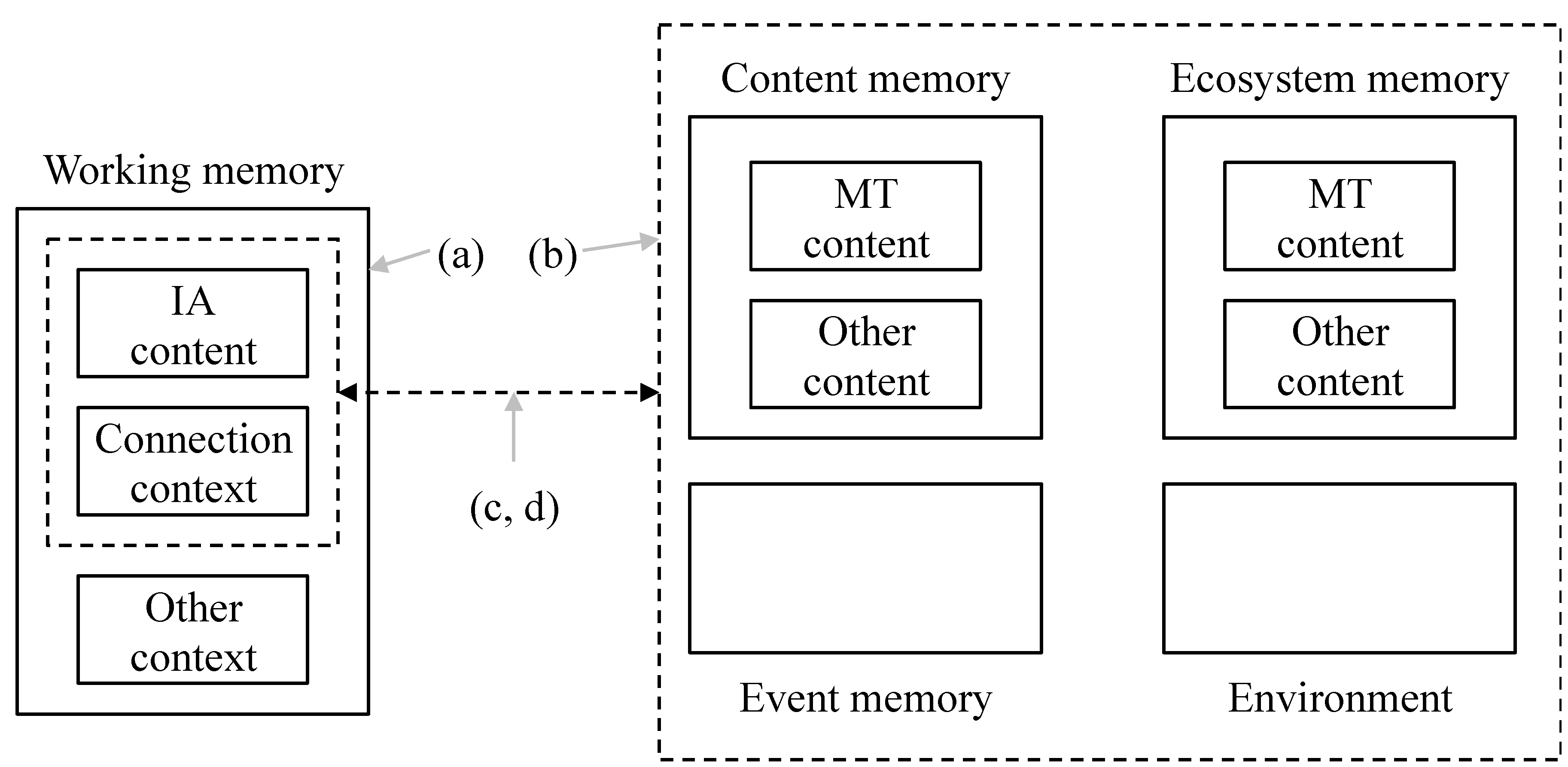
In order to make an interpretation, an IE has to recognise the content in an IA by connecting it to what is in memory. The interpretation depends critically on the connections stored in working memory and their links to other memories. In making these connections there may be many options. A selection from these options forms the (recognition) connection strategy, shown in Figure 1. (Although it is concerned with recognition, since no other connection strategies are discussed in this paper it is known as the connection strategy in the rest of the paper.)

Figure 1. Recognition connection strategy.

Figure 1. Recognition connection strategy.

The Figure shows the following connection strategy factors:

(a)

Context: as well as the IA under consideration, how much else of the external environment is taken into account?

(b)

Search space: there are choices about how widely to look. An IE can look in various subsets of content memory or event memory. It can look elsewhere in the Ecosystem or more generally in the environment.

(c)

Options: how many options will be entertained? Is the first good enough or are all of them needed?

(d)

Success threshold: when is a connection good enough to qualify for the interpretation? Is there any kind of quality threshold that must be met?

The result of the connection strategy is a set of connected content in working memory with further connections into memory (references to Ecosystem content and the environment are stored in content and event memory).

The connection strategy trades off IQ and IF (see [1]). Figure 2 shows the range of possibilities for each factor of the connection strategy shown in Figure 1.

Figure 2. Connection strategy factors.

Figure 2. Connection strategy factors.

Consider these factors in turn. The context defines how much the IE tries to recognise—is it just the IA or is it the IA in its context. For example, if A is talking to B, does B consider just what A is saying or also take into account A’s current emotional state, what other people are saying and so forth.

When processing an IA the minimum sensible search space is that containing the content in the IA. At the other extreme, a thorough search will also consider much more. So, a computer query may just search for the string “John” but a person may also consider other stored attributes of various Johns (second name, address, whereabouts etc.) that may be relevant to the search. The search space also depends on the Modelling Tool in use. A particular Modelling Tool (e.g., Mathematics) may naturally limit the search space to connections directly concerned with the Modelling Tool.

The option factor is straightforward—does the IE just accept the first match, or require several, or all. The success threshold defines what constitutes a match—is there a quality standard that needs to be met in terms of the nature of the connections or related to derivation. This is clearly related to Action IQ. An element of the success threshold is coherence. The importance of coherence for an IE is clear—without a coherent interpretation of the environment it will not be possible effectively to evaluate courses of action (and their potential relationship with outcomes). In [8], Kahneman describes how “associative memory, …, continually constructs a coherent interpretation of what is going on in our world at any instant”. As Kahneman makes clear, coherence is not necessarily linked to other aspects of quality.

The ability to recognise and make connections is clearly important to humans, animals and computers. At an organisational level, the importance is captured in the title of [9]—“If only HP knew what HP knows”.

A limited connection strategy may be less reliable, but given the combinatorial difficulties of more extensive strategies, may be much more efficient to implement. The connection strategy factors demonstrate the scale of the combinatorial problem—the more thorough the search the greater the level of resources needed. So, it is natural that selection processes have resulted in a trade-off between efficiency and quality. Consider human beings as an example. Kahneman [8] describes what he calls System 1 and System 2 and indicates the imperfections that apply to humans. He says:

“…most of what you (your System 2) think and do originates in your System 1, but System 2 takes over when things get difficult, and it normally has the last word. … System 1 has biases, however, systematic errors that it is prone to make in specified circumstances.”

“System 1 is radically insensitive to both the quality and quantity of information that gives rise to impressions and intuitions.”

As a result, we cannot reliably trust our System 1 (but often do so without realising it).

Systems 1 and 2 provide examples of generic connection strategies for humans—we can call them connection strategy abstraction patterns. System design and programming define connection strategies for computer programs. In general, elements of the connection strategy will be defined or constrained by:

• the abstraction pattern of an IE (e.g., DNA, system architecture);
• the history of interactions of an IE (e.g., education, market success);
• the elements of an IA.

Connection strategy defines how much resource to apply and how good the answer needs to be (although neither of these may be apparent to the IE). So it is one of the key outcomes of selection processes.

Connection strategy is complicated, sometimes well hidden and has a major impact on IQ, so it makes sense that different Ecosystems have developed different approaches to assessing its effectiveness. Consider, for example:

• questions and answers (in conversation);
• cross-examination (in the legal process);
• peer review (in the academic world);
• thought and introspection.

These help answer the question: what level of IQ is appropriate for an Ecosystem?

But can we assume that the particular Modelling Tool corresponding to an Ecosystem is the most appropriate for providing the levels of IQ needed by the Ecosystem? The invention of Mathematics and, more recently, computer modelling suggests that the answer is “no” in some cases but outside a few Ecosystems the question is not necessarily addressed.

3.2. Derivation

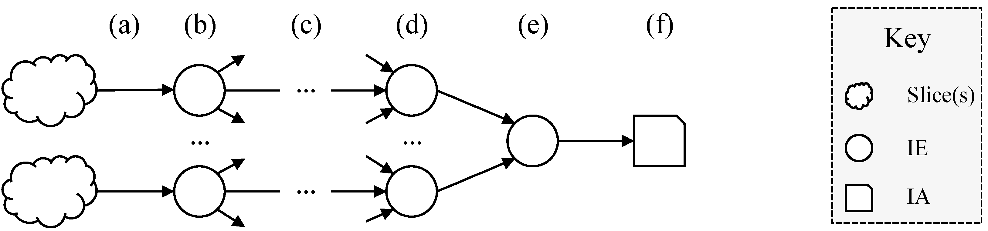
Figure 3 shows the overall process by which an IA is derived.

Figure 3. Derivation.

Figure 3. Derivation.

The figure shows the stages of the derivation of an IA, as follows:

(a)

Measurement process: possibly at many different times and using many different measurement processes relating to different Ecosystems a number of properties of slices are measured;

(b)

Processing by an IE: each IE (potentially amongst many) senses and analyses the input and then creates one or more IAs;

(c)

Transmission: the IAs can be transmitted on various channels and in various modes (e.g., one-to-one or one-to-many);

(d)

Processing: intermediate IEs may convert between Ecosystems, combine IAs or process them in other ways;

(e)

Combination: one such IE produces the final IA (f).

The whole process may be extremely complicated and may cross Ecosystem boundaries many times (e.g., between people and computers). There are many ways in which quality may degrade and different Ecosystems have devised different ways of dealing with it. For example:

• in IT, there are rigorous processes for designing, building and testing systems [10]—ensuring that the subsequent derivation of information is robust;
• in legal processes there are rules for handling evidence so that information presented in court has a reliable derivation;
• scientists pay considerable attention to the design of experiments so that measurement is as reliable as possible.

Other types of Ecosystem may be less scrupulous.

4. Measures

In this section we define the various measures related to different types of content. First a review of some definitions, mostly drawn from [1].

4.1. Definitions

Content in Modelling Tools is of the following types:

• atom: the fundamental indivisible level of content in the Modelling Tool (note that this definition is different from the definition of “atom” in [11]);
• chunk: groups of atoms;
• assertion: the smallest piece of content that is a piece of information—containing two chunks in a manner that conforms to an assertion abstraction pattern;
• passage: a related sequence of assertions.

For the sections below and using the definitions established in [1], suppose that:

• M is a Modelling Tool (and all of the subsequent definitions are with respect to M);
• Γ_Μ is the set of content in M;
• Γ_γΜ is the set of chunk content in M and γ, δ ∈ Γ_γΜ;
• Γ_αΜ is the set of assertion content in M and α, β ∈ Γ_αΜ where α = (γ, ρ, δ) and ρ is an assertion abstraction pattern;
• Γ_πΜ is the set of passage content in M and π ∈ Γ_πΜ;
• Ξ is the set of set theoretic relationships;
• Σ is the set of all slices;
• T is a set of discrete times and t ∈ T;
• φ_γ: Γ_γΜ × T → 2^Σ, is a chunk interpretation; Φ_γ is the set of all chunk interpretations (for M);
• φ_α: Γ_αΜ × T → 2^Σ × Ξ × 2^Σ, is an assertion interpretation; Φ_α is the set of all assertion interpretations (for M);
• φ_π: Γ_πΜ × T → f (2^Σ, …, 2^Σ), is a passage interpretation where f is a Boolean expression (containing ANDs); Φ_π is the set of all passage interpretations (for M);
• φ_eγ, φ_eα, φ_eπ are the corresponding the Ecosystem interpretations.

4.2. Chunks, Assertions, Passages and Interpretations

Chunks and assertions are different kinds of content. Chunks specify constraints and assertions make hypotheses about the relationship between different constraints. The interpretations of chunks correspond to sets created using the following operators to create the constraints: ∩, ∪, \, ^c (where A^c is the absolute complement of A). By contrast, interpretations of assertions use set containment and equality comparisons (⊆, ⊇, ⊂, ⊃, =, ≠).

The definition of interpretations in Section 4.1 is general but we are only interested in interpretations that correspond to an IE or Ecosystem. From now on the term interpretation will be restricted to just that: interpretation by an IE or Ecosystem. Any IE, at any time, will have a unique interpretation of any chunk, assertion or passage.

There are relationships between the different types of assertion. Any assertion interpretation induces two chunk interpretations. But note that the assertion provides a context for the chunks that may change the chunk interpretations. An example is provided by the psychological biases that Kahneman refers to in [8]. For passages, the situation is more complex. The same chunk may occur more than once and be interpreted in different ways each time. This is the issue addressed by the measure “precision” addressed below.

Interpretations may not be well behaved. In the most general case an interpretation may be unrelated to the structure of an assertion or passage (as implied by the Modelling Tool). For example, the interpretation of some French by someone who does not understand French grammar may be well wide of the mark. In general, selection pressures will drive IE interpretations towards that of the Ecosystem. So we want to consider interpretations that are close, in some sense, to the Ecosystem interpretation and that respect the following structures and Ecosystem behaviour of the Modelling Tool:

• the relations implicit in the assertion;
• synonyms (i.e., chunks for which the interpretation is the same);
• discrimination (i.e., chunks for which the interpretation is different).

In each case we have to allow the actual interpretations to be different, but we want the structure to remain the same. So, if φ is a passage interpretation, which induces corresponding chunk and assertion interpretations, define:

• the φ-closure of γ, σ_φ(γ) = {δ ∈ Γ_γΜ: φ (δ, t) = φ (γ, t)};
• the closure of γ, σ(γ) = {δ ∈ Γ_γΜ: φ_e (δ, t) = φ_e (γ, t)};
• Γ_σΜ = {σ(γ): γ ∈ Γ_γΜ};

and say that

• φ is MT-closed if σ(γ) = σ_φ(γ) for all γ ∈ Γ_γΜ;
• φ is MT-structured if φ maps to the same relation as φ_e for all passages;
• φ is MT-consistent if φ is MT-closed and MT-structured.

4.3. Boolean Passages

Suppose that α and β are assertions. Consider the statements:

• α OR β;
• IF α THEN β.

It may not be possible for an IE to interpret them in the manner described above—depending on the IE they do not necessarily correspond to the satisfaction of one or more constraints (although an IE may process them as if they were). In some sense there is information missing. If α and β refer to the same chunk (as in “the cat was black” OR “the cat was grey”) then they correspond to a single assertion (“the cat was black or grey"). But in the most general case (“the cat was black” OR “the dog was old”) this is not possible.

They are clearly useful in terms of selection processes both with respect to the current environment state (e.g., “there is a gust of wind over there or a large animal is moving the grass”) or outcomes (e.g., “if it is a large animal then I am in danger”). An IE may have access to the “missing” information in memory but it makes sense to distinguish between recognition and assessment [1]. Recognition is about interpreting the environment state on its own; assessment is about combining that interpretation with other information in memory to decide what action to take. For the purposes of this paper interpretation is concerned with recognition.

Within MfI there are two ways to address such statements depending on whether we are dealing with one Modelling Tool or two. Assume first of all that the Boolean operators are part of the same Modelling Tool as the assertions. Define a Boolean passage to include such statements. As with a passage, we can say that interpretation of a Boolean passage corresponds to Boolean expression of interpretations of assertions (with the caveat that the interpretation of chunks may vary throughout the Boolean expression). Each assertion and passage is a Boolean passage. Call the set of Boolean passages Γ_βΜ.

Now suppose we are dealing with two Modelling Tools: one (M₁) for the assertions (perhaps a language) and another (M₂) that includes the Boolean operations and Boolean expressions. Such an IA is described as a Composite IA [1]. In this case, the complexity raised above does not arise. In M₂, the chunks are M₁ assertions (as in “IF P AND Q THEN R” in which P, Q and R are chunks for M₂). In this case, there is a chance that the two Modelling Tools are interpreted independently and the results combined separately. This distinction corresponds to a question raised by Popper in [12] that is discussed in Section 5. In terms of the connection strategy discussed above, the search space may well be different if two Modelling Tools are involved rather than just one.

This discussion shows how the model can be extended to non-Boolean passages. Suppose M_n is a set of Modelling Tools that support a range of non-Boolean operations and expressions. Composite IAs produced from M_n will allow different overall interpretations depending on the degree to which the interpretations from the different Modelling Tools are combined (or not). This leads to the question: what is the effect on IQ if the different interpretations are independent or in different combinations? This approach may enable an analysis of complex, recursive passages or generalisations of Popper’s question. This is a topic for further research.

We can extend the definitions of MT-structured and MT-consistent to the interpretations of Boolean passages in the obvious way. For the rest of the paper, unless otherwise notified, it is assumed that all interpretations are MT-consistent.

4.4. Measures for Chunks—Accuracy

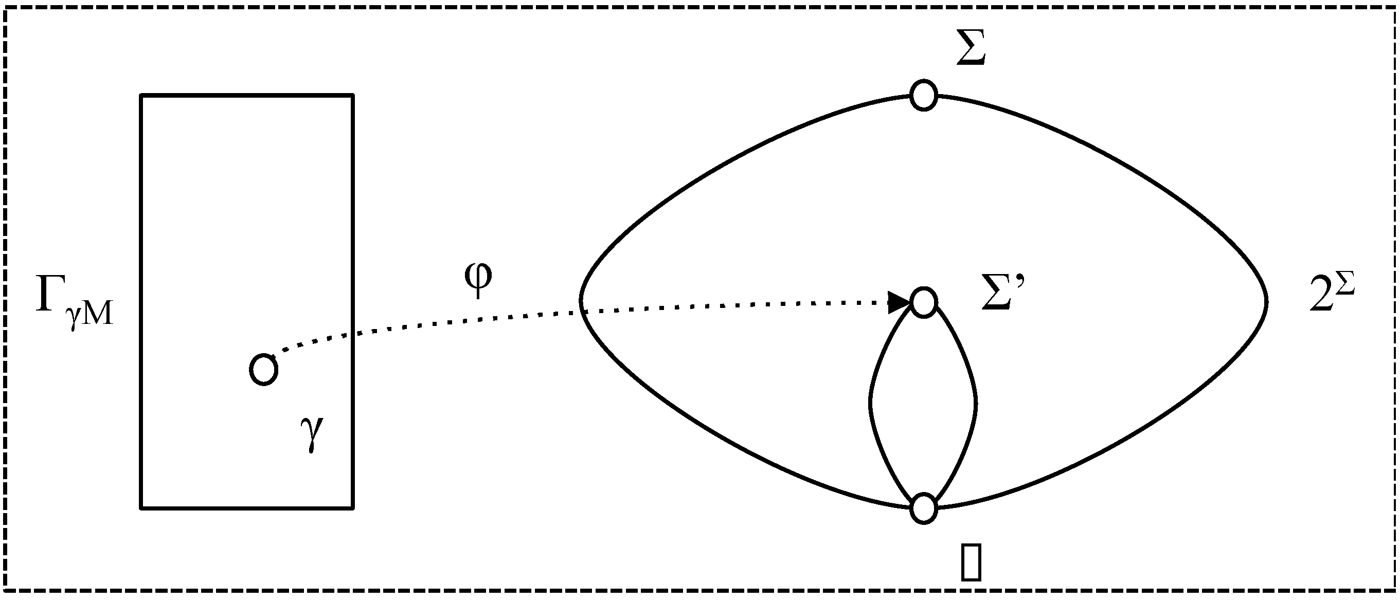
At any given time, chunk interpretations map chunk content to a subset of slices as shown in Figure 4 in which φ maps γ to Σ’. The right hand side of the diagram shows the partial order on 2^Σ induced by set inclusion and the corresponding partial order on Σ’.

Figure 4. Chunk interpretation.

Figure 4. Chunk interpretation.

Assume that φ_e is the Ecosystem interpretation and φ, φ' are chunk interpretations. For chunks, we can define the following:

• φ is γ-accurate (with respect to t) if φ (γ, t) = φ_e (γ, t) ≠ ∅;
• φ is γ-inaccurate (with respect to t) if φ (γ, t) ∩ φ_e (λ, t) = ∅ ;
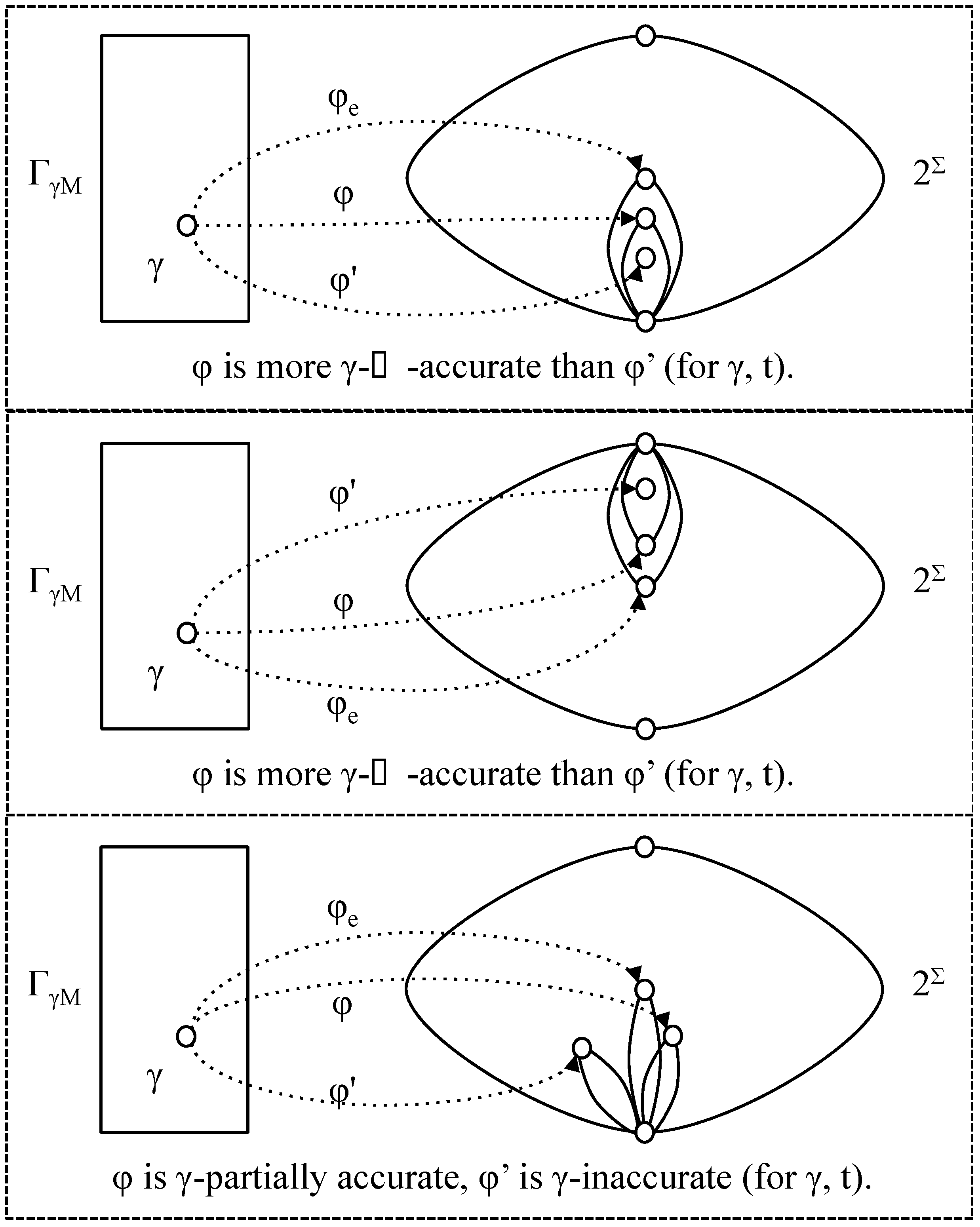
• φ is more γ-⊂-accurate than φ' (with respect to t) if φ' (γ, t) ⊂ φ (γ, t) ⊆ φ_e (γ, t);
• φ is more γ-⊃-accurate than φ' (with respect to t) if φ_e (γ, t) ⊆ φ (γ, t) ⊂ φ' (γ, t);
• φ is more γ-accurate than φ' (with respect to t) if it is more γ-⊂-accurate or more γ-⊃-accurate (note that it cannot be both);
• φ is γ-partially accurate (with respect to t) if φ (γ, t) ∩ φ_e (λ, t) ≠ ∅ and φ (γ, t) φ_e (λ, t) ≠ ∅.

The definitions can be extended (and “γ-” removed) by insisting that they apply for all γ ∈ Γ_γΜ. Figure 5 shows some of these definitions diagrammatically. We can use these definitions to compare interpretations. Define:

• φ <_acc,t φ' if φ' is more accurate than φ;
• φ =_acc,t φ' if φ = φ';
• ≤_acc,t, >_acc,t, ≥_acc,t correspondingly.

≤_acc,t is anti-symmetric—suppose that

• φ <_acc,t φ' and φ' ≤_acc,t φ; then
• φ ≠_acc,t φ' and there is some γ for which (depending on the type of relative accuracy) either

  • φ (γ, t) ⊂ φ' (γ, t) ⊆ φ_e (γ, t), or
  • φ_e (γ, t) ⊆ φ' (γ, t) ⊂ φ (γ, t).

In either case it cannot be true that φ' ≤_acc,t φ. So ≤_acc,t provides a partial order for Φ_γ for any time t (other partial order requirements are guaranteed by set inclusion).

Figure 5. Relative accuracies.

Figure 5. Relative accuracies.

4.5. Measures for Chunks—Precision

Assume that T’ ⊆ T is a time interval and that φ is an interpretation that applies at (potentially) multiple times to chunks during T’. Define:

• the ∩_T’-range of φ with respect to γ, ∩_T’-ran (φ, γ) = {σ: σ ∈ φ (γ, t) ∀ t ∈ T’};
• the ∪_T’-range of φ with respect to γ, ∪_T’-ran (φ, γ) = {σ: ∃ t ∈ T’ such that σ ∈ φ (γ, t)};
• φ is γ-precise (with respect to T’) if ∩_T’-ran (φ, γ) = ∪_T’-ran (φ, γ);
• φ is γ-imprecise (with respect to T’) if ∩_T’-ran (φ, γ) = ∅;
• φ is more γ-precise than φ' (with respect to T’) if

  • ∩_T’-ran (φ, γ) ⊃ ∩_T’-ran (φ', γ) and ∪_T’-ran (φ, γ) ⊆ ∪_T’-ran (φ', γ), or
  • ∩_T’-ran (φ, γ) ⊇ ∩_T’-ran (φ', γ) and ∪_T’-ran (φ, γ) ⊂ ∪_T’-ran (φ', γ);
• φ is as γ-precise as φ' (with respect to T’) if

  • ∩_T’-ran (φ, γ) ⊇ ∩_T’-ran (φ', γ) and ∪_T’-ran (φ, γ) ⊆ ∪_T’-ran (φ', γ).

The definitions can be extended (and “γ-” removed) by insisting that they apply for all γ ∈ Γ_γΜ. Again we can compare interpretations. Define:

• φ <_pre,T’ φ' if φ' is more precise than φ' for time period T’;
• φ =_pre,T’ φ' if φ = φ';
• ≤_pre,T’, >_pre,T’, ≥_pre,T’ correspondingly.

≤_pre,T’ is anti-symmetric because if φ is more γ-precise than φ' then it cannot be true that φ' is as γ-precise as φ. So ≤_pre,T’ is a partial order for Φ_γ.

Precision applies to interpretations of the same content at different times. This may include multiple instances of the same piece of content in the same passage. In this case, as in others, the context may determine that the different interpretations should be different—that, according to the interpretation, they are intended to refer to different sets of slices. In this case, we need to narrow the measures to groups of chunks, i.e., sets of chunks that, according to the Ecosystem conventions that apply to the Modelling Tool, are intended to refer to the same thing. When we apply precision to the interpretation of a Boolean passage, the period T’ will (usually) be a very short interval and we can write ≤_pre,[t] instead of ≤_pre,T’.

4.6. Measures for Chunks—Coverage

Coverage is an attribute of the Modelling Tool (note that the definition here is different to the definition in [1]). Coverage captures the number of properties of slices that are incorporated in a chunk and how tightly the value constrains the property. This relates directly to the syntax of the Modelling Tool. So, for example, “two metre tall, dark-haired man” has more coverage than “tall, dark-haired man” and, in turn, this has more coverage than “tall man”. We can define:

• γ >_cov γ’ if γ has greater coverage than γ';
• ≥_cov, ≤_cov, <_cov correspondingly.

If γ and γ’ are synonyms (or the equivalent in other Modelling Tools) then γ ≤_cov γ’ and γ’ ≤_cov γ and we cannot deduce that γ = γ’. But if we define the set

• σ’(γ) = {δ ∈ Γ_γΜ: γ ≤_cov δ and δ ≤_cov γ}

then ≤_cov is a partial order for Γ_σ’Μ = {σ’(γ): γ ∈ Γ_γΜ}. In this case we clearly have σ’(γ) ⊆ σ(γ). But the definition of exact synonyms is that they are interpreted in the same way so σ᾽(γ) = σ(γ).

4.7. Measures for Chunks—Resolution

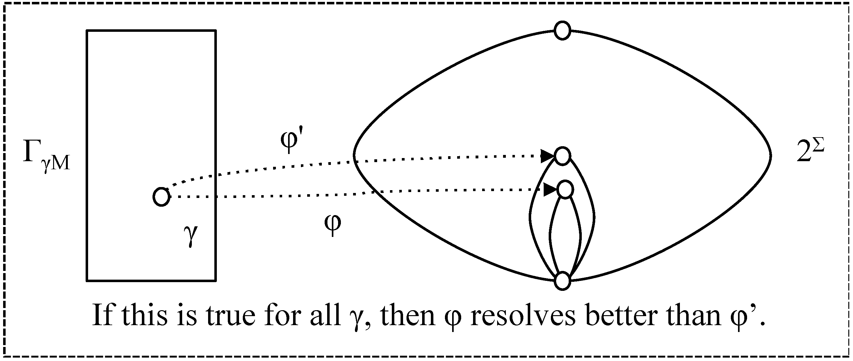
Greater coverage provides the potential to discriminate between alternative environment states. Resolution measures the extent to which the interpretation supports discrimination. Say that

• φ resolves as well as φ' (with respect to t) if for all γ ∈ Γ_γΜ, φ (γ, t) ⊆ φ' (γ, t); (note that this is a different definition from that in [1] but it expresses the concept more clearly).

Figure 6 illustrates the concept of resolution.

Figure 6. Resolution.

Figure 6. Resolution.

Define:

• φ ≤_res,t φ' if φ resolves as well as φ' (for t);
• ≥_res,t, <_res,t, >_res,t correspondingly.

Then, ≤_res,t is a partial order for Φ_γ. (As before, by insisting that resolution applies to all chunks we can guarantee that ≤_res,t is anti-symmetric.)

4.8. Measures for Chunks—Timeliness

Timeliness is a measure of a different type. It measures the difference between the time of measurement of properties and the time of interpretation. In this case it is a total order that is independent of content and interpretation and that we can call ≤_tim.

4.9. Measures for Chunks—Overall

Partial orders can be combined in a number of ways to create further partial orders, but there are two specific mechanisms of interest here: sum and product. Suppose that A and B are disjoint sets, ≤_a1 and ≤_a2 are partial orders on A, ≤_b is a partial order on B and C = A × B. Define:

• a ≤_a a’ if a ≤_a1 a’ and a ≤_a2 a’ for a, a’ ∈ A;
• c ≤_c c’ if a ≤_a1 a’ and b ≤_b b’ for c = (a, b), c’ = (a’, b’), a, a’ ∈ A, b, b’ ∈ B.

Then ≤_a is the sum of ≤_a1 and ≤_a2 and ≤_c is the product of ≤_a1 and ≤_b and both are partial orders. Table 1 lists the orders described above and some combinations.

Table 1. Combined chunk partial orders.

Order	Definition	Assumes	Applies to
≤acc,t	As above	Fixed t	Φγ
≤pre,T’	As above—precision applies to interpretations of all instances of a chunk in the time period in question	Range T’	Φγ
≤res,t	As above	Fixed t	Φγ
≤cov	As above	-	Γσ
≤tim	As above	-	T
≤cq,t	sum (≤acc,t, ≤res,t)	Fixed t	Φγ
≤ci,t	product (≤cov, ≤res,t)	Fixed t	ΓσΦγ = Γσ × Φγ

Table 1. Combined chunk partial orders.

Order	Definition	Assumes	Applies to
≤acc,t	As above	Fixed t	Φγ
≤pre,T’	As above—precision applies to interpretations of all instances of a chunk in the time period in question	Range T’	Φγ
≤res,t	As above	Fixed t	Φγ
≤cov	As above	-	Γσ
≤tim	As above	-	T
≤cq,t	sum (≤acc,t, ≤res,t)	Fixed t	Φγ
≤ci,t	product (≤cov, ≤res,t)	Fixed t	ΓσΦγ = Γσ × Φγ

≤_cq,t measures the quality of the interpretation of a chunk. ≤_ci,t measures both the coverage of a chunk (≤_cov) and how much of that potential has been converted in the interpretation (≤_res,t).

4.10. Measures for Assertions

The quality of assertions depends both on the quality of the relevant chunks and the quality of the relation with respect to the chunk interpretations. In that sense, an assertion is a hypothesis that different interpretations may confirm or refute. So assume that α = (γ, ρ, δ) is an assertion and

• φ (α, t) = (φ (γ, t), r, φ (δ, t)).

We can say that:

• α is (not) φ-plausible (with respect to t) if r (φ (γ, t), φ (δ, t)) is (not) satisfied;
• α is (not) plausible (with respect to t) if r (φ_e (γ, t), φ_e (δ, t)) is (not) satisfied.

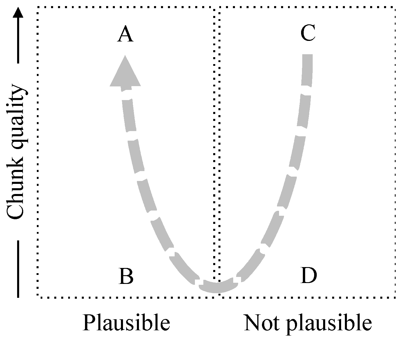
The relationship between plausibility and chunk quality is shown in Figure 7. The vertical axis relates to the chunk quality and assumes that the two chunks are of comparable quality but, with that caveat, it shows some interesting zones marked A, B, C and D. (The vertical axis is only indicative since chunk quality is a partial order not a total order.)

Figure 7. Plausibility and chunk quality.

Figure 7. Plausibility and chunk quality.

Zone A represents assertions that are most likely to be true (in an Ecosystem sense)—plausible and supported by high chunk quality. Zone C represents assertions that can be considered contradictions—those that have a relation that does not correspond to a reliable (high quality) relation between the chunks. Zones B and D correspond to low chunk quality and are correspondingly unreliable. The dotted line shows increasing reliability of plausibility (or perhaps we should call it trustworthiness).

Table 2 shows how orders for chunks can be extended to assertions.

Table 2. Orders for assertions.

Order	Definition	Applies to
≤cq,[t]	sum (≤pre,[t], ≤acc,t, ≤res,t)	Φγ
≤aq,[t]	product (≤cq,[t], ≤cq,[t])	Φγ × Φγ
≤ai,[t]	product (≤ci,t, ≤ci,t)	ΓσΦγ × ΓσΦγ

Table 2. Orders for assertions.

Order	Definition	Applies to
≤cq,[t]	sum (≤pre,[t], ≤acc,t, ≤res,t)	Φγ
≤aq,[t]	product (≤cq,[t], ≤cq,[t])	Φγ × Φγ
≤ai,[t]	product (≤ci,t, ≤ci,t)	ΓσΦγ × ΓσΦγ

In the order ≤_cq,[t] in the table, the [t] subscript in ≤_pre,[t] denotes that precision is measured over all of the chunks in a group in the assertion. This measure is of relatively little value for assertions but will assume a greater importance when we consider passages below.

Any assertion interpretation induces two chunk interpretations and, for the last two rows, the third column in the Table represents the corresponding chunk interpretations. The second order (≤_aq,[t]) measures the quality of the chunks in the assertion but still just works in the direction of the y-axis in Figure 7. The final order (≤_ai,[t]) measures the overall coverage and resolution of the chunks in the assertion.

None of these orders captures the impact of plausibility (for which the objective is to mimic the dotted line in Figure 7) so consider the following definitions:

• P = Γ_αΜ × Φ_α × T;
• P_αt0 = {φ ∈ Φ_α: α is not φ-plausible (with respect to t)} and similarly P_αt1 for which α is φ-plausible;
• P_αt = P_αt0 ∪P_αt1.

For any fixed α, t, P_αt0 and P_αt1 are disjoint, so define ≤_ar,α[t] as follows:

• if φ, φ' ∈ P_αt0, then φ ≤_ar,α[t] φ' if φ ≥_aq,[t] φ';
• if φ, φ' ∈ P_αt1, then φ ≤_ar,α[t] φ' if φ ≤_aq,[t] φ';
• if φ ∈ P_αt0 and φ' ∈ P_αt1, then φ <_ar,α[t] φ'.

Then ≤_ar,α[t] is a partial order that enables the comparison of the reliability of plausibility between different interpretations of the same assertion.

4.11. Measures for Boolean Passages

For Boolean passages, we can define another measure based on the number of assertions in the Boolean passage. Suppose

• β₁ = f (α_1i) is a passage and α_1i = (γ_1i, ρ_1i, δ_1i);
• β₂ = f (α_2j) is a passage and α_2j = (γ_2j, ρ_2j, δ_2j);

then define

• β₁ ≤_na β₂ if α_1i∈ {α_2j for all j} for all i.

In this case β₂ is constructed from a superset of the assertions in β₁.

Table 3 shows how we can use a similar approach to combine orders as for assertions.

Table 3. Orders for Boolean Passages.

Order	Definition	Applies to
≤na	As above	Γβ
≤pcov	product (≤cov, …, ≤cov)	Γβ
≤pc	sum (≤na, ≤pcov)	Γβ
≤pq,[t]	product (≤cq,[t], …, ≤cq,[t])	Φβ
≤pi,[t]	product (≤ci,[t], …, ≤ci,[t])	ΓσnΦβn = ΓσΦγ× … × ΓσΦγ
≤pi2,[t]	product (≤na, ≤pi,[t])	Γβn× ΓσnΦβn
≤pu,[t]	product (≤pc, ≤pq,[t])	Γβn× Φβn

Table 3. Orders for Boolean Passages.

Order	Definition	Applies to
≤na	As above	Γβ
≤pcov	product (≤cov, …, ≤cov)	Γβ
≤pc	sum (≤na, ≤pcov)	Γβ
≤pq,[t]	product (≤cq,[t], …, ≤cq,[t])	Φβ
≤pi,[t]	product (≤ci,[t], …, ≤ci,[t])	ΓσnΦβn = ΓσΦγ× … × ΓσΦγ
≤pi2,[t]	product (≤na, ≤pi,[t])	Γβn× ΓσnΦβn
≤pu,[t]	product (≤pc, ≤pq,[t])	Γβn× Φβn

The table suggests that ≤_pcov applies to Γ_β, but how can this be if two Boolean passages are of different sizes? Strictly, ≤_pcov applies to Γ_σ× … × Γ_σ but two projections map Γ_β first to Γ_γ× … × Γ_γ then to Γ_σ× … × Γ_σ so we can apply ≤_pcov to Γ_β. Now suppose that β₁, β₂ are Boolean passages with β₁ larger than β₂ (in the sense that it contains more assertions) and β₁₁ is the initial piece of β₁ that corresponds to the size of β₂. Then define ≤_pcov for β₁, β₂ as follows:

• if β₁₁ ≥_pcov β₂ then β₁ >_pcov β₂;
• if β₁₁ <_pcov β₂ then β₁ and β₂ are not comparable;
• if β₁₁ and β₂ are not comparable then β₁ and β₂ are not comparable.

Coverage increases with the number of chunks but quality decreases so the same idea applies in reverse to the quality-related orders. Define ≤_pq,[t] for β₁, β₂ as follows:

• if β₁₁ ≤_pq,[t] β₂ then β₁ <_pq,[t] β₂;
• if β₁₁ >_pq,[t] β₂ then β₁ and β₂ are not comparable;
• if β₁₁ and β₂ are not comparable then β₁ and β₂ are not comparable.

Finally, how does this apply to ≤_pi,[t] and ≤_pu,[t]? In this case, coverage increases with the number of chunks but quality does not, so we need to restrict comparison to Boolean passages of the same size (in terms of assertions). This is denoted by the n suffix in the third column of Table 3.

Plausibility can be extended similarly. Suppose that:

• β = f (α_i);
• α_i = (γ_i, ρ_i, δ_i);
• φ (α_i, t) = (φ (γ_i, t), r_i, φ (δ_i, t)), where r_i corresponds to ρ_i;

then say that

• β is (not) φ-plausible (with respect to t) if f (r_i (φ (γ_i, t), φ (δ_i, t))) is (not) satisfied;
• β is (not) plausible (with respect to t) if f (r_i (φ_e (γ_i, t), φ_e (δ_i, t))) is (not) satisfied.

This definition of plausibility can be used to define the reliability of plausibility (or φ-plausibility, similarly) for Boolean passages in the same way as for assertions. Consider the following definitions:

• Q = Γ_βΜ × Φ_β × T;
• Q_βt0 = {φ ∈ Φ_β: β is not φ-plausible (with respect to t)} and similarly Q_βt1;
• Q_βt = Q_βt0 ∪ Q_βt1.

For any fixed β, t, Q_βt0 and Q_βt1 are disjoint, so define ≤_pr,β[t] as follows:

• if φ, φ' ∈ Q_βt0, then φ ≤_pr,β[t] φ' if φ ≥_pq,[t] φ';
• if φ, φ' ∈ Q_βt1, then φ ≤_pr,β[t] φ' if φ ≤_pq,[t] φ';
• if φ ∈ Q_βt0 and φ' ∈ Q_pt1, then φ <_pr,β[t] φ'.

Then ≤_pr,β[t] is a partial order that enables the comparison of the reliability of plausibility between elements of Q_βt.

These orders are preorders not partial orders since anti-symmetry no longer applies.

4.12. Restricting Measures

A limitation of the approach described above is that the measures for accuracy, precision and resolution rely on the properties of interpretations for all chunks. If two interpretations vary in relative quality for different subsets of chunks then they will not be comparable. This corresponds, for example, to the situation in which two people have different areas of expertise.

This limitation is caused by the scope of the chunks. The measures apply only to a single Modelling Tool so we may decide that the different areas of expertise correspond to different, more specific, Modelling Tools. But, more generally, we can apply the measures to subsets of chunks so long as what remains is rich enough to support the ability to create Boolean passages. In this way we can create measures that focus in on specific areas of interest.

4.13. Summary of Orders

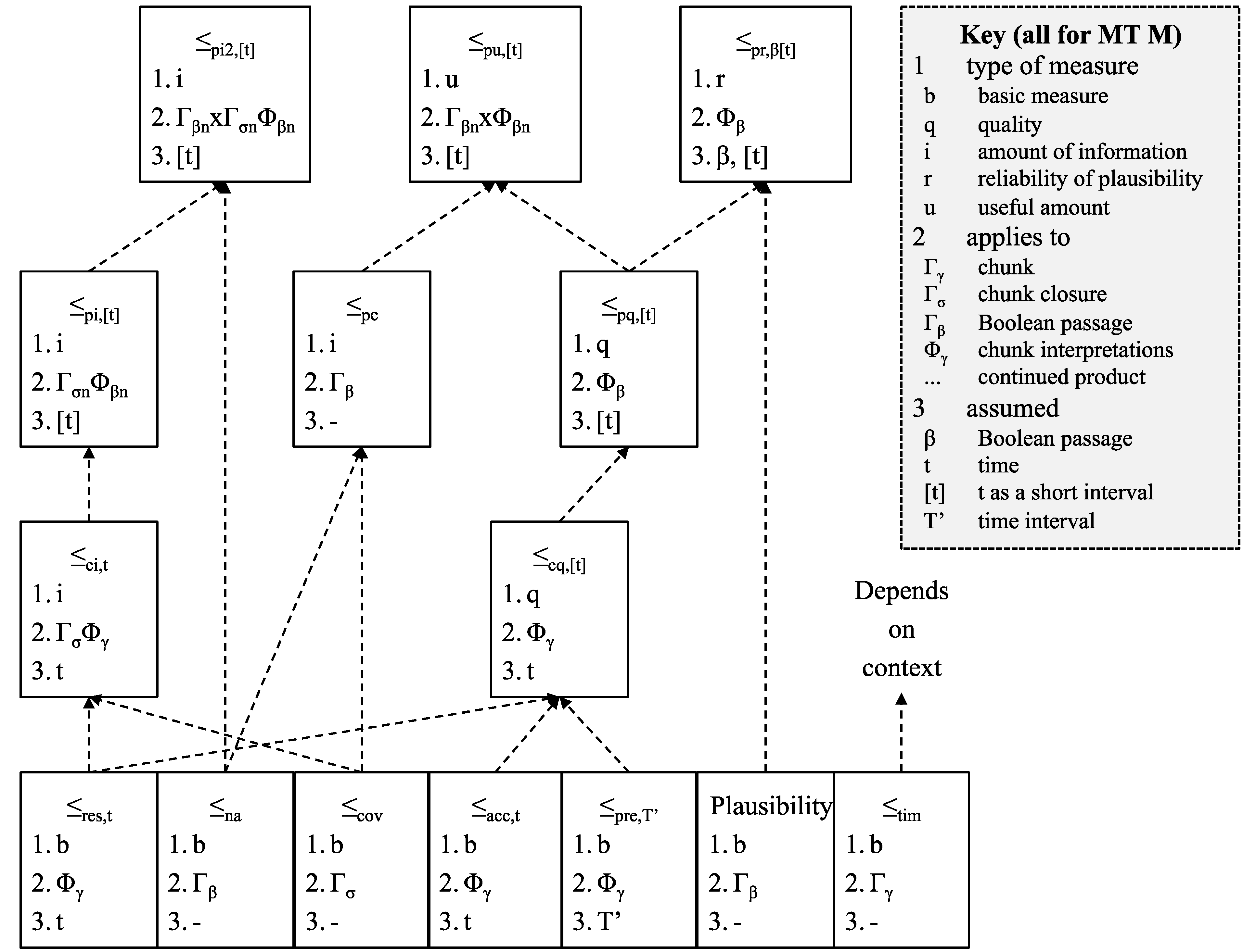
Figure 8 summarises the relationship between some of the orders defined above.

Figure 8. Relationship between orders.

Figure 8. Relationship between orders.

The Figure shows how basic measures (at the bottom) can be combined into measures like the reliability of plausibility and the useful amount of information. Timeliness may play a role depending on usage (this is discussed further in Section 5 below).

5. Truth and Truthlikeness

In [2], Floridi reviews important questions in the Philosophy of Information and asks “can information explain truth”? He adds the following supplementary questions:

“Whether an informational theory could explain truth more satisfactorily than other current approaches” and

“if that is answered in the negative, whether an informational approach could at least help to clarify the theoretical constraints to be satisfied by other approaches.”

MfI allows truth to be examined from a number of different viewpoints and supplies some constraints (of the type that Floridi refers to). Truth is expressed using IAs and IAs are interpreted by IEs. So, truth (for an IE) is related to both an IA and its interpretation and the nature of truth cannot be disentangled from the quality of information. There are several implications of this.

First, interpretation may be unreliable. In Section 3 above, we discussed the difficulties that humans have in handling information because they are liable to psychological biases [8]. So we cannot wholly rely on our perceptions of truth.

Now consider the geometry of information. The measures described above generally only support partial orders or preorders. This means that, overall, information cannot support many-valued logics [13] that assume that truth-values satisfy a total order.

Within an Ecosystem, the perception of truth is the result of Ecosystem conventions. This is consistent with [14] in which, according to Kuhn, even the most rigorous of human activities (science) relies on consensus in the relevant community. He discusses a paradigm in the following terms:

“I mean to suggest that some accepted examples of scientific practice—examples which include law, theory, application, and instrumentation together—provide models from which spring coherent traditions of scientific research.”

The “accepted examples” and “coherent traditions” he mentions correspond to Information Ecosystems.

The Ecosystem concept in MfI reinforces the view of [11,15] that information is relative—that it relies on Ecosystem conventions at one level and the specific interpretation of an IE at the next. Indeed, within MfI, the interpretation of “truth”, like that of all concepts, is Ecosystem-dependent, so we would expect different approaches to the subject of truth.

Popper [12] introduced an example of this when he suggested that a statement can be logically true but also falsifiable as a statement about the world. His example was “2 apples + 2 apples = 4 apples”. The first interpretation (“logically true”) relies on connections only using the conventions of the Modelling Tool (Mathematics in this case). In the terms of Figure 2, the context is the IA only, the search space is Modelling Tool content only and the Modelling Tool only defines the success threshold. By contrast, the second interpretation allows a wider connection with events in the world. To make the same point another way, the first uses Mathematics as the Modelling Tool and the second uses both language and Mathematics and subjects the connection to a more rigorous connection assessment. The distinction between the two is a demonstration of the difference between pure Mathematics and science. But it also demonstrates that, if truth is concerned with reality in the physical world then conclusions reached on the basis of a limited connection strategy alone may well be unreliable.

For his example, it is easy to see that the interpretations coincide fairly readily. However if we consider the example “2 piles + 2 piles = 4 piles” then it is more difficult. The second form of interpretation depends on what “+” means since it is also possible that “2 piles + 2 piles = 1 pile” (or other numbers). In this case the quality of the assertion is reduced.

The subsequent sections develop the implications of the relativity of information for truth and truthlikeness. Truth corresponds to the reliability of plausibility and the discussion below shows that truthlikeness can also be explained using the same measure.

5.1. Measures of Information—Truth

Truth is expressed using information but, more specifically, using Boolean passages. What does this mean for “the truth, the whole truth and nothing but the truth”? Truth itself is defined by the relevant Ecosystem interpretation and, in terms of the measures defined above, it corresponds to high reliability of plausibility (≤_pr,β[t]). This criterion corresponds to those used in different Ecosystems including, for example:

• the law—“beyond reasonable doubt”;
• science—for example, the six-sigma criterion used in particle physics experiments like the test for the Higgs boson.

As we find with these and other Ecosystems, it may not be possible to assess these tests without a robust connection strategy and reliable derivation.

Truth may also be concerned with timeliness, depending on the usage. An interpretation may have been true at the time an IA was created but no longer true at the time of the interpretation. It is a matter of convention and usage whether the word “true” applies to the time of the creation of an IA, the time of its interpretation or some other time. But, if required, we can also include the timeliness order ≤_tim or some variant of it.

The whole truth poses a new challenge—is there anything missing? The simple answer is that there always will be. It is impossible to capture the entire state of a slice—this is the “blind men and the elephant” point discussed, for example, in [16]. The whole truth is linked to the “amount of information” discussed below and so, for intrinsic IQ, the whole truth is impossible to achieve.

But we can analyse the whole truth in relation to action IQ. The main difference between intrinsic IQ and action IQ is that, in the latter case, it is possible (theoretically) to determine what is sufficient to resolve the possible alternatives. This is determined by coverage (is there enough “breadth” of information?) and resolution (how much is interpreted?) as well as the number of relations that need to be satisfied (the number of assertions). So we can use ≤_pi2,[t].

Finally, nothing but the truth requires that the Boolean passage does not include any chunks γ for which the interpretation is less γ-⊃-accurate than Ecosystem interpretation.

5.2. Measures of Information—Truthlikeness

Truthlikeness is discussed in [2]. In Section 5.1 we considered part of this question: to what extent can we compare interpretations of a Boolean passage with respect to reliability of plausibility. In this section we consider the extent to which Boolean passages can be truthlike and the extent to which can we define progressively truthlike Boolean passages.

A simple example first—suppose that a room contains 150 people. Then (assuming a reasonable interpretation):

(1)

“the room contains 150 people” is plausible;

(2)

“the room contains about 150 people” is also plausible;

(3)

“the room contains 151 people” is implausible but close (in some sense).

In this case by varying the value of a single property we can change the interpretation of the assertion from implausible to plausible. In particular the coverage of the relevant chunk decreases from 1 to 2 and then increases again from 2 to 3.

We can generalise from this example using the concept of reliability of plausibility. If we relax and then tighten the degree of coverage then we may be able to trace a sequence from an implausible passage to a plausible passage so that the reliability of plausibility increases along the sequence. If this is possible then we can say that the degree of truthlikeness increases along the path. In this sense, reliability of plausibility becomes a measure of truthlikeness. We can formalise this in the following way. Consider the following definitions:

• P = Γ_αΜ × Φ_α × T;
• pl: P → {0, 1} where “0” represents “not plausible” and “1” represents “plausible”;
• α_i = (γ, ρ, δ_i) for 1 ≤ i ≤ n where the δ_i correspond to values for a single property and Α = {α_i};
• Q_t0 = {α_i∈ Γ_αΜ: pl (α_i, φ_e, t) = 0} and similarly Q_t1;
• Q_t = Q_t0 ∪ Q_t1.

Suppose Α’ = {α’₁, α’₂, α’₂}, Α’ ⊆ Α and Α’ has the following property:

• α’₁ >_cov α’₂ <_cov α’₃;
• α’₁∈ Q_t0;
• α’₂, α’₃∈ Q_t1.

Then the definition of Α’ mirrors the technique in the above example. It may be possible to compare the proximity of assertions. Suppose that:

• α ∈ Q_t0;
• α’₁ >_cov α >_cov α’₂ <_cov α’₃.

Then α is “closer” to reliable plausibility than α’₁. And a corresponding statement applies if:

• α ∈ Q_t1;
• α’₂ <_cov α <_cov α’₃.

The reliability of plausibility order enables a comparison of different interpretations. The relaxation and tightening of coverage (as above) enables some pairs of assertions to be compared.

6. The Amount of Information

The amount of information is a measure that has caused difficulties. In both the Bar-Hillel-Carnap paradox (BCP) [3] and the scandal of deduction [4], definitions of the amount of the amount of information have caused counter-intuitive results and different approaches have been taken to resolution (see, for example, the discussion in [2]). In this section we apply the ideas developed throughout the paper and show that MfI provides a natural way to treat the amount of information.

In both cases, the discussion follows the same course. The BCP and scandal of deduction are both intuitively unsatisfactory because the previous definitions of the “amount” of information do not reflect the relativity and constraints of information. When these are added, using the definitions of measures of information above and the approach of MfI more generally, the paradox and scandal disappear.

6.1. The Bar-Hillel Carnap Paradox (BCP)

In [2] Floridi describes the Bar-Hillel-Carnap paradox (BCP) in the following way:

“According to the classic quantitative theory of semantic information, there is more information in a contradiction than in a contingently true statement.”

So the BCP leads to the following questions:

• what does “more information” refer to?
• what is a contradiction?
• what does it mean in terms of MfI and the measures above?

Figure 8 shows some ways of treating the “amount of information”. For chunks (using the order ≤_ci,t), the amount of information relates to the degree to which the chunks constrain and how well the constraint is resolved in interpretation. Chunks can be combined into ever more constraining specifications. For assertions and Boolean passages it is also a question of volume—how many assertions form the Boolean passage (using the order ≤_na). These can be combined for Boolean passages (in the order ≤_pi2,[t]).

Because chunks can be defined in Modelling Tools independently of reality they can over-constrain with the result that interpretations map to the empty set. This is the MfI equivalent of a part of the BCP but it applies to chunks only, which cannot be contradictions (they are constraints, not statements about constraints), and in this case the quality of such a chunk (in terms of ≤_cq,t) is low.

A contradiction is a Boolean passage that is implausible with high quality. This can never be the case for a Boolean passage containing an over-constrained chunk.

The amount of information is a term that combines measures of chunks, the number of assertions and interpretations. If we include quality we can consider the “useful” amount of information. The order ≤_pu,[t] defined in Table 3 includes these elements (although it uses ≤_pc rather than ≤_pi2,[t] because resolution is already taken into account in ≤_pq,[t]).

So, using the tools of MfI, there is no paradox and we can refine the notion of the amount of information by including quality in a measure of the useful amount of information.

6.2. The Scandal of Deduction

In [17] D’Agostino describes the “scandal of deduction” as follows:

“According to the received view, logical deduction never increases (semantic) information. This tenet clashes with the intuitive idea that deductive arguments are useful just because, by their means, we obtain information that we did not possess before.”

This is discussed further in [18,19]. When the scandal of deduction is viewed through the lens of MfI it prompts a number of questions including, for example, the following:

• “Logical deduction never increases (semantic) information”—for whom?
• What does increased information mean?

Approaching the issue from an interpretation of an IA by an IE, we can frame the question in terms of MfI. Suppose that the following is true: “P IMPLIES Q” (we assume, here, that “true” means reliably plausible, as above, for a particular Ecosystem). Then we need to consider whether, under these circumstances, there is more information in P and Q than in P. More information can mean more information in an IA, more in the memory of an IE or a combination of the two. This means that there are a number of possibilities to consider.

There are shown in Table 4 that considers the options when an IE interprets an IA. In all cases the IA contains at least “P” and never contains “Q”. The options numbered 1–8 in Table 4 are analysed below.

Table 4. Options for the amount of information.

α1 = “P” α2 = “P IMPLIES Q” α3 = “Q”		IE memory contains…
		-	α2	α3	α2, α3
IA contains…	α1	1	2	3	4
	α1, α2	5	6	7	8

Table 4. Options for the amount of information.

α1 = “P” α2 = “P IMPLIES Q” α3 = “Q”		IE memory contains…
		-	α2	α3	α2, α3
IA contains…	α1	1	2	3	4
	α1, α2	5	6	7	8

The connection strategy determines how thorough the process of recognition is and the creativity, rigour and extent of processing determines the subsequent analysis. (We are assuming, for example, that the IE cannot prove “P IMPLIES Q” if it is not provided.) So, all we can say is that there are a number of possibilities depending on these two factors. But if we stick to the possibilities that arise naturally out of Modelling Tool processing then there are the following:

(a)

the IE makes a connection with the content during recognition (depending on the connection strategy) but does not store the content in memory;

(b)

the content is stored in memory as a result of recognition (as a by-product of the Modelling Tool processing, again depending on connection strategy);

(c)

the content is stored in memory as a result of processing (again depending on the nature of the processing).

In each case, the amount of information may mean one or both of the following:

• the amount in the IA;
• how much is added to the memory of the IE and, in particular, whether either or both of the following are added (assuming that “P” is added in each case):

  ○

  “P IMPLIES Q”;

  ○

  “Q”.

These possibilities, applied to the options contained in Table 4, are shown in the columns of Table 5. In the last two columns a, b, and c refer to the corresponding possibilities in the list above.

Table 5. The amount of information.

Option	Amount of information in IA	Possibility that “P IMPLIES Q” added	Possibility that “Q” added
1	Less	No	No
2	Less	No	c
3	Less	No	No
4	Less	No	No
5	More	a, b	a, b, c
6	More	No	a, b, c
7	More	a, b	No
8	More	No	No

Table 5. The amount of information.

Option	Amount of information in IA	Possibility that “P IMPLIES Q” added	Possibility that “Q” added
1	Less	No	No
2	Less	No	c
3	Less	No	No
4	Less	No	No
5	More	a, b	a, b, c
6	More	No	a, b, c
7	More	a, b	No
8	More	No	No

An analysis of coverage and the number of assertions confirms that there is more information in the IA (designated “More”) in options 5–8 than in 1–4 (“Less”) as shown in the second column of the table. The subsequent columns indicate the content that may be added to the memory of the IE (in some cases, it is already there). The table demonstrates that there is no scandal of deduction in this case.

If we add an analysis of quality then the result shown in Table 5 is not so straightforward. If α₁, α₂ are not reliably plausible then α₃ is not a reliable deduction.

The discussion so far has been for an IE but exactly the same applies to an Ecosystem as a whole. But, of course, the implication is also that connections made by logical deduction form part of the conventions of the Ecosystem.

In [6], Burgin says that: “the information in a message is a function of the recipient as well as the message.” Logan reviews the relativity of information in [9] and concludes that: “information is not an absolute but depends on the context in which it is being used.” The approach of MfI supports this assertion, so we can naturally deduce, as Table 5 shows, that the amount of information is a relative concept—it is relative to combination of IAs and IEs (and Ecosystem) in question.

7. Conclusions

The underlying model (MfI) presented in [1] supports measures of the quality and amount of information. In this paper these, and derived, measures have been used to analyse and integrate a number of measures of information previously proposed in the literature including truth, truthlikeness and the amount of information. The combined set of measures provides an integrated framework for measuring information in which some of the traditional difficulties (e.g., the Bar-Hillel Carnap paradox and the scandal of deduction) can be avoided.

References

- Walton, P. A Model for Information. Information 2014, 5, 479–507. [Google Scholar] [CrossRef]
- Floridi, L. The Philosophy of Information; Oxford University Press: Oxford, UK, 2011. [Google Scholar]
- Bar-Hillel, Y.; Carnap, R. An Outline of a Theory of Semantic Information. 1953. Reproduced in Language and Information: Selected Essays on Their Theory and Application; Addison-Wesley: Reading, MA, USA, 1964. [Google Scholar]
- Hintikka, J. Logic, Language-Games and Information: Kantian Themes in the Philosophy of Logic; Clarendon Press: Oxford, UK, 1973. [Google Scholar]
- Avgeriou, P.; Uwe, Z. Architectural patterns revisited: A pattern language. In Proceedings of 10th European Conference on Pattern Languages of Programs (EuroPlop 2005), Bavaria, Germany, July 2005.
- Burgin, M. Theory of Information: Fundamentality, Diversity and Unification; World Scientific Publishing: Singapore, 2010. [Google Scholar]
- Tulving, E. Episodic and semantic memory. In Organization of Memory; Tulving, E., Donaldson, W., Eds.; Academic Press: New York, NY, USA, 1972; pp. 381–403. [Google Scholar]
- Kahneman, D. Thinking, Fast and Slow; Macmillan: London, UK, 2011. [Google Scholar]
- Sieloff, C.G. “If only HP knew what HP knows”: The roots of knowledge management at Hewlett-Packard. J. Knowl. Manag. 1999, 3, 47–53. [Google Scholar] [CrossRef]
- Sommerville, I. Software Engineering; Addison-Wesley: Harlow, UK, 2010. [Google Scholar]
- Kohlas, J.; Schmid, J. An Algebraic Theory of Information: An Introduction and Survey. Information 2014, 5, 219–254. [Google Scholar] [CrossRef]
- Ryle, G.; Lewy, C.; Popper, K.R. Symposium: Why are the calculuses of logic and arithmetic applicable to reality? In Logic and Reality, Proceedings of the Symposia Read at the Joint Session of the Aristotelian Society and the Mind Association at Manchester, United Kingdom, 5–7 July 1946; pp. 20–60.
- Gottwald, S. Many-Valued Logic. The Stanford Encyclopedia of Philosophy. Zalta, E.N., Ed.; Spring 2014 ed. Available online: http://plato.stanford.edu/archives/spr2014/entries/logic-manyvalued/ (accessed on 26 January 2015).
- Kuhn, T.S. The Structure of Scientific Revolutions. Enlarged, 2nd ed.; University of Chicago Press: Chicago, IL, USA, 1970. [Google Scholar]
- Logan, R. What Is Information?: Why Is It Relativistic and What Is Its Relationship to Materiality, Meaning and Organization. Information 2012, 3, 68–91. [Google Scholar] [CrossRef] [Green Version]
- Brenner, J. Information: A Personal Synthesis. Information 2014, 5, 134–170. [Google Scholar] [CrossRef]
- D’Agostino, M. Semantic Information and the Trivialization of Logic: Floridi on the Scandal of Deduction. Information 2013, 4, 33–59. [Google Scholar] [CrossRef]
- D’Alfonso, S. On Quantifying Semantic Information. Information 2011, 2, 61–101. [Google Scholar] [CrossRef]
- Finger, M.; Reis, P. On the Predictability of Classical Propositional Logic. Information 2013, 4, 60–74. [Google Scholar] [CrossRef]
© 2015 by the authors; licensee MDPI, Basel, Switzerland. This article is an open access article distributed under the terms and conditions of the Creative Commons Attribution license (http://creativecommons.org/licenses/by/4.0/).
Share and Cite
MDPI and ACS Style
Walton, P. Measures of Information. Information 2015, 6, 23-48. https://doi.org/10.3390/info6010023
AMA Style
Walton P. Measures of Information. Information. 2015; 6(1):23-48. https://doi.org/10.3390/info6010023
Chicago/Turabian StyleWalton, Paul. 2015. "Measures of Information" Information 6, no. 1: 23-48. https://doi.org/10.3390/info6010023