 Wenyi Wang
 Juanjuan Zheng
 Lihong Song
 Yukun Tu
 Peng Gao
- 1School of Computer and Information Engineering, Jiangxi Normal University, Nanchang, China
- 2School of Education, Jiangxi Normal University, Nanchang, China
One purpose of cognitive diagnostic model (CDM) is designed to make inferences about unobserved latent classes based on observed item responses. A heuristic for test construction based on the CDM information index (CDI) proposed by Henson and Douglas (2005) has a far-reaching impact, but there are still many shortcomings. He and other researchers had also proposed new methods to improve or overcome the inherent shortcomings of the CDI test assembly method. In this study, one test assembly method of maximizing the minimum inter-class distance is proposed by using mixed-integer linear programming, which aims to overcome the shortcomings that the CDI method is limited to summarize the discriminating power of each item into a single CDI index while neglecting the discriminating power for each pair of latent classes. The simulation results show that compared with the CDI test assembly and random test assembly, the new test assembly method performs well and has the highest accuracy rate in terms of pattern and attributes correct classification rates. Although the accuracy rate of the new method is not very high under item constraints, it is still higher than the CDI test assembly with the same constraints.
Introduction
The theory of cognitive diagnostic assessment (CDA) is an important part of personalized adaptive learning (Sia and Lim, 2018). Since the cognitive diagnostic model (CDM) was put forward, it has attracted much attention because of its ability to analyze and explain the test results in detail (Hsu et al., 2020). On the other hand, the test is the bridge between the abstract and unobservable ability of the examinees and the real observable item response data, so the quality of the test affects the quality of diagnostic classification directly. A test that meets the test specification needs to be selected from an item bank, then the test assembly will be restricted by many conditions and requirements (Zijlmans et al., 2019; Tang and Zhan, 2020), such as the difficulty and discrimination under the constraints of psychometrics, the maximum number of knowledge points allowed in a test, or the requirements of parallel tests.
How to construct a test with higher quality has always been a research hotspot. In the aspect of test assembly based on cognitive diagnosis, the test assembly method of CDM information index (CDI) proposed by Henson and Douglas (2005) is of great influence. Henson et al. (2008) put forward the attribute level discrimination index (ADI) under uniform and non-uniform distribution of attributes. However, neither the CDI method nor the ADI method considers the attribute hierarchical structure. When these methods are applied in practice, the performance of CDI and ADI methods will be poor under some conditions if the hierarchical structure exists between attributes (Kuo et al., 2016). In addition, Finkelman et al. (2009) proposed a method of test assembly based on genetic algorithm minimizing the expected posterior error rate for attributes under the framework of CDA. For example, the method of test assembly based on genetic algorithm takes three fitness functions: the average number of classification errors, maximum error rate, and ability to hit attribute-level target error rates. This method can directly optimize the classification errors, but its computational intensity is considerably greater than that of analytic procedures like the CDI. For classroom or formative assessment, we should choose the algorithm with low computational complexity if other algorithms for test assembly are sufficient to meet the needs (Clark, 2013).
In terms of test assembly methods based on cognitive diagnosis, researchers have proposed a large number of methods, but most of these methods are based on a certain CDI, and there are some problems such as lacking of global consideration or requiring large amount of computation. Therefore, it is urgent to consider the global information and the method of test assembly with less calculation in cognitive diagnosis. The method of test assembly based on CDI takes into account the sum of the whole amount of information, but it has been found that this method is not the optimal method of test assembly. In some cases, the total amount of information is the largest, which may due to some of the larger information on a non-trivial subset of the universal set of latent classes (i.e., the set of all possible combinations of attributes). The discriminating power of this strategy with the largest CDI is not necessarily better than the strategy with uniform distribution of information and less overall information. Therefore, the goal of this study is to explore a new method for test construction, and combine the idea of cluster analysis (Guo et al., 2020) and mixed-integer linear programming method (Kantor et al., 2020) to propose a method to maximize the minimum distance (MMD) between latent classes, in order to overcome the shortcomings of the existing methods.
Methods
Cognitive Diagnostic Model
The purpose of cognitive diagnostic model is to describe the relationship between examinee’s item response and his or her potential cognitive attributes (Mao, 2014). It is a psychometric model. The common cognitive diagnostic models are the deterministic input noisy “and” gate (DINA) model, the deterministic input noise “or” gate (DINO) model, and the reduced-reparameterized unified model (R-RUM; Hartz, 2002). The new method proposed in this study mainly focused on these two cognitive diagnosis models. Let K be the number of attributes to be measured by the test. The entry qjk in the Q-matrix indicates whether the attribute k is measured in item j. When qjk = 1, the attribute k is measured by item j. And 0 indicates that it has not been measured. αik indicates the attribute status of examinee i, that is, 1 indicates examinees’ mastery of attribute k, and otherwise 0.
The DINA model is a completely non-compensatory model, which requires that the examinees must master all the attributes required by the item for correctly answering. As long as any one of them is not mastered, it will lead to a wrong answer or a very low probability of correct answer. For the value of the ideal response , a value of 1 indicates that the examinee i has mastered all the attributes measured by the item j, while a value of 0 means that the examinee has not fully mastered the attributes measured by the item j. The corresponding probabilities of correct answer to this item are (1−sj) and gj respectively. The formula of DINA model is as follows (Junker and Sijtsma, 2001)
The DINO model is the compensatory model. As long as the examinees have mastered any of the attributes measured by the item, they can have a higher probability of correctly answering. For the value of the ideal response is 1, it means that the examinees have mastered at least one attribute measured by item j. A value of 0 indicates that the examinees have not mastered all the attributes of item j. The formula of the DINO model is as follows (Templin and Henson, 2006)
where sj is the slip probability for the examinees of the ideal response with value 1 on item j, and gj is the guessing probability for the examinees with value 0 on item j.
Like the DINA model, R-RUM is a non-compensatory model, which is a simplified unified model of reparameterization. The baseline parameter indicates the positive response probability for examinees who have mastered all the attributes required by item j. The values are all between 0 and 1. The penalty parameter for not possessing the kth attribute is defined at the level of interaction between the item and the attributes and reflects the importance of attribute k on item j. The formula of R-RUM is as follows (Hartz, 2002)
For simplify, the correct answer probability P(Xij = 1|αi) is denoted by Pj(αi), where αi is the knowledge state of the examinee i.
Kullback-Leibler Information Distance Between Classes
Considering the existing cognitive diagnosis item bank, attribute vectors of all items in the item bank have been specified (Wang et al., 2020), and the parameters of each item have been estimated by the parameter estimation algorithm of cognitive diagnosis model. The correct answer probability Pj(αc) of knowledge state αc on item j can be calculated by item attribute vector qj and item parameters, where αc is a knowledge state of the examinees and is an element of the universal set of latent classes. Let M be the size of the item bank. Kullback-Leibler (K-L; Cover and Thomas, 2006; Debeer et al., 2020) information quantity or K-L distance is the most commonly used to measure the distance between any two probability distributions Pj(αu) and Pj(αv) for two knowledge states αu and αv. Formally, item j is defined as the K-L distance of the item response probability distributions under the knowledge states of αu and αv
In fact, DK–L is the expectation of the function of the logarithmic likelihood ratio of probability distributions Pj(αu) and Pj(αv). Although this amount of information is called the distance between the two distributions, and it does have statistical significance for distance measurement, that is, with the increase of DK–L, it is easier to distinguish the two distributions statistically (Rao, 1962). But it is not symmetrical, that is, DK−L(αu,αv)≠DK−L(αv,αu).
Kullback-Leibler distance is often used for computer adaptive testing or cognitive diagnostic computer adaptive testing. For instance, Chang and Ying (1996) firstly suggested that K-L distance instead of Fisher information should be used as a more effective item selection index in computer adaptive testing based on one-dimensional IRT model. Madigan and Almond (1995) use K-L distance for test selection strategy of belief networks. Tatsouka and Ferguson (2003) use K-L distance and Shannon entropy for sequential item selection and use it in cognitive diagnostic computer adaptive testing. Different from the amount of Fisher information, the K-L distance does not require that the parameter space must be continuous, so it is suitable for CDM where the attribute pattern is discrete.
Test Assembly Using Mixed-Integer Linear Programming
In cognitive diagnosis, the probability of correct answer or the expected vector of item response of knowledge state αc on test length of J in a test isP(αc) = (P1(αc),P2(αc),…,PJ(αc)). For knowledge state αc, the P(αc) can be regarded as the center of the class. In pattern recognition or clustering methods, the method of maximum distance between classes can usually be used for classification. If the cognitive diagnostic test can maximize the distance between the class centers of all potential classes αc ∈ Qs, where Qs is the universal set of latent classes, it is easier to classify knowledge states. It is just like in a jigsaw puzzle, if there is a big difference between the sub-images, the difficulty of completing the puzzle will be correspondingly lower.
In order to characterize the distinguishing power of item j to knowledge states αu and αv, the following is DK–L as its metric index. For any αu and αv, the discrimination power matrix or K-L distance matrix Dj = (D(αu,αv,j)) is obtained. If the cardinality (i.e., the number of elements) of Qs is T, we know that the number of rows or columns is T in Dj. In order to use the mixed-integer linear programming for test construction, it is necessary to vectorize the matrix Dj into a single stacked column vector. That is, the sequence of rows in this matrix is composed of a long vector, and then transpose the row vector to get the stacked column vector, which is denoted as Vj = Vec(Dj). When the matrix Dj is vectorized, we remove the main diagonal elements because these values are zeros. For each item in the item bank, Vj can be calculated, and the matrix V = (V1,V2,…,VM) composed of all the items can be obtained, where M is the number of items in the item bank. Based on the mixed-integer linear programming model, we will give a linear programming model which takes into account the mean value of the distance between all classes and maximizes the minimum distance between classes:
Subject to
xj ∈ {0,1}, j = 1, 2, …, M,
Among them, f1 = (f11,f12,…,f1M)T, where . The negative of f1j is used to convert a maximization problem into a minimization one. Here, is the weight of y, x = (x1x2…xM)T, where x1x2⋯xM is the 0-1 vector in the decision vector of linear programming, and the value of the xj indicated whether the test contains the item j. If xj = 1, it means that the test contains the item j, otherwise it does not include the item j, b = (b1,b2,…,bT(T−1))T represents the lower limit of K-L distance for all pairs of knowledge states. You can set the bounded distance , which is the average value of the distance between classes of J items in the item bank. 1Tx = J represents the test length constraint, where 1Tis a M-dimensional column vector with all elements 1, and J is the test length. y captures the difference between the t-th pair inter-class distance V(t)x and the target distance bt, where V(t)is row t in V. Then, adding y to the constraint condition, and adding f2y to the objective function, is to maximize the minimum inter-class distance y. For example, if the components in b are equal, and V(t)x is the smallest of all the distances between classes, if V(t)x < bt, then V(t)x can at least add bt−V(t)x to satisfy the constraint. Because the average distance between other classes is larger than V(t)x, V(t)x needs to add bt−V(t)x to reach the constraint. And minimizing f2y in the objective function is minimizing f2(bt−V(t)x). Because f2y is positive and bt fixed, that is maximizing V(t)x which is the minimum inter-class distance between classes. In the objective function, we also consider the f1x, linear programming model at the same time, that is, to maximize the distance between all classes, because the model also contains 0-1 vector x and real vector y, so this linear programming model is a typical mixed-integer or mixed 0-1 linear programming model, which can be solved by intlinprog function in Matlab2015a. For the source codes, we provided a user-friendly code in MATLAB into a public repository at the website: https://github.com/JXNU-EduM/MMD-Test-Assembly-for-CD/.
Simplify of K-L Distance Matrix
The distance indexDK−L in this study needs to be calculated for mixed-integer linear programming, so it is necessary to process the distance index matrix with vectorizing, transposing and merging. In the case of no hierarchical structure of attributes, there are T = 2K possible mastery modes for K attributes, and there are M items in the item bank. The size of the distance matrix of M items on the 2K attribute mastery patterns after vectorizing, transposing and merging is M*2K(2K−1). If M is 300 and K is 4, the size of the distance matrix is 300∗240. Although the size of the matrix is within the acceptable range, the amount of calculation for mixed-integer linear programming is a little large, so if possible, the distance matrix should be simplified.
If the u-th row and v-column element in Dj is denoted by Djuv, and the corresponding element in Vj is denoted by Vjuv. Djuv or Vjuv is the discriminating power for these two different knowledge states of αu and αv, and one condition for the smallest difference between the two knowledge states is that there is a k-th attribute in the two attribute mastery patterns, which makes the k-th attribute mastery status of the two patterns different, and all mastery status except k are exactly the same. If only the discriminating power among attribute patterns with the least difference for the item is considered when vectorizing the distance matrix, the Vjuv can be simplified. In the following, the distance matrix index corresponding to the simplified Vjuv is recorded as SDK−L. According to the characteristics of attribute patterns, we know that if the number of attributes is K and a certain attribute pattern is given, there are K attribute patterns with the least difference from it. Because of the asymmetry of the distance between αu and αv, that is, the DK−L distance from αu and αv is different from that from αv to αu, both Djuv and Djvu should be considered. If the number of attributes is three and the attributes are independent and without hierarchical structure, there are eight possible attribute mastery patterns, as shown in Figure 1: the difference of attribute patterns with connections between adjacent levels is the smallest. Thus, only 24 elements needed to be considered in Dj is obviously smaller than the number of non-diagonal elements in Dj, which can greatly save the computational cost.

Figure 1. Partial relation for eight possible attributes mastery patterns.
Study Design
Some main factors that may affect the efficiency of constructing test assembly should be considered: cognitive diagnosis model (the DINA model, the DINO model, and the R-RUM), attribute correlation coefficient (0 and 0.5), the number of examinees was fixed at 10000, the size of item bank was fixed at 300, the number of measured attributes was fixed at 4. Attribute correlation coefficient is zero, implying that the attributes were independent of each other, and the knowledge state was distributed evenly. Under each condition, the experiment was repeated for 200 times.
Assuming that the test measured K attributes, there are at most 2K−1 possible item attribute vectors. First of all, all possible item attribute binary vectors were converted to decimal as 1, 2,…, 2K−1, and then 300 random integers in the range [1, 2K−1] were randomly generated. Item attribute vectors of 300 items with corresponding numbers were selected to form the Q-matrix for an item bank. Item parameters of each item were randomly generated from specified distributions. The DINA and DINO models have the guessing and slip item parameters, which are randomly generated from a uniform distribution U (0.05, 0.4). Meanwhile the R-RUM also has the baseline and penalty parameters, which are respectively randomly generated from the uniform distribution U (0.75, 0.95) and U (0.2, 0.95). These were the same as the experimental design of Henson and Douglas (2005).
When the examinees are simulated, two aspects need to be considered: one is attribute mastery status αki at the k-th attribute for the i-th examinee and the other is the correlation coefficient between attributes, denoted by ρ. Multivariate normal distribution can be used to simulate latent ability, , where 0 is the zero vector with the length of K and Σ is the correlation matrix
In this study, the value of ρ is 0 (independent structure) or 0.5. After getting the value of , we need to discretize it. The strategy of discretization of αki is
Two groups of 10000 examinees were simulated. One group of examinees was used to calculate the empirical distribution of knowledge state, which will be applied as the prior distribution for compute the posterior mode in the classification of the other group. We have not changed this condition for the repetition of the study of Henson and Douglas (2005). If a lager sample is available for the calibration of item bank, the empirical distribution of attribute patterns from the large sample will be applied as the prior distribution to computing the posterior mode in the classification of examinees who have taken the tests constructed from the calibrated item bank.
For a set of given attribute mastery pattern, PXij = 1|αi depending on the selected model is the probability of correct response to item j for examinee i with attribute mastery pattern αi. We supposed u was randomly generated from a uniform distribution U (0, 1). The item response of the ith examinee on item j can be obtained by discretizing the probability matrix
Since the item parameters were known, the examinees’ item responses on the selected items could be simulated, and then the examinees were classified by maximum posterior estimation, and then attribute correct rate (ACR) and pattern correct rate (PCR) could be calculated. The formulas of ACR and PCR are as follows
and
In the above two expressions, N and K represent the number of examinees and the number of attributes, respectively, and I(x = y) is an indicative function, which is defined as follows: when x = y, I(x = y) = 1, otherwise it is 0. The attribute correct rate (ACR) is the proportion of examinees whose estimated attribute status is equal to the simulated or true attribute status, while the pattern correct rate (PCR) is the proportion of examinees whose estimated attribute patterns is equal to the simulated or true attribute patterns. These two indices are commonly used in the simulation study for evaluating the correct classification rates for attributes or attribute patterns. The higher PCR and ACR for a test construct method implies that it yields considerably higher correct classification rates.
The DK–L distance was used as the inter-class distance, and the mixed-integer linear programming is used to maximize the minimum inter-class distance with additional constraints. The test length is 20 for all test design. The first constraint was no constraint (No Constraints, NC), which directly used the greedy algorithm to construct test, and did not set any constraints based on the CDI or MDD. The second constraint was item-level constraint (Item Constraints, IC), which controls the number of items that measure a specific number of attributes for test assembly. According to the suggestion of Henson and Douglas (2005), among the 20 items that measure a total of 4 attributes, 9 items measured three attributes, 7 items measured two attributes, and the remaining 4 items measured one attribute. The third constraint was the attribute number constraint (Attribute Constraints, AC), which required that each attribute must be measured at least 7 times in a test with four attributes and 20 items.
Study 1: Comparison Between the Proposed Method and Its Simplification
The proposed method uses mixed-integer linear programming to maximize the minimum inter-class distance between classes and comprehensively to consider the overall amount of information in order to achieve better test assembly quality. However, when the number of attributes measured was four, the calculation of the distance matrix DK−L after vectorizing by the new method was a bit large, so when using the new method to construct test assembly, the distance matrix needs to be simplified. The test assembly method using the original and simplified matrices were denoted by DK−L and SDK−L, respectively. In fact, the simplification of the distance matrix will reduce the constraints of mixed-integer linear programming. The simplified matrix aims to discriminate similar attribute patterns, but whether it will lose the amount of information, if it is true, the size of the loss still needs to be verified.
Research Purpose
The purpose of this study is to verify whether the simplified distance matrix will lose information and lead to poor results. Since this study only considered the effect of simplified constraints on the efficiency of the MMD test assembly method, a single factor or one-way analysis of variance (ANOVA) can be performed on the two groups of ACR and PCR before and after the simplification in order to measure the impact of simplified constraints on ACR and PCR. In addition, the mean of ACR or PCR before and after simplification and the index of constructing test assembly time (in seconds) need to be taken into account.
Experimental Steps
In order to achieve the purpose of this study, the experiment was designed according to the following steps:
(1) According to the design of Section 3 (four attributes were considered), we simulate two groups of examinees, in which one group was used to calculate the prior distribution, and the other group was used for classification. We simulate the Q matrix and item parameters in the item bank, and simulate the observed complete item response matrix of all examinees on all items in the item bank.
(2) Calculate the DK−L distance and the simplified DK−L distance of all items on all possible attribute mastery patterns.
(3) Choose the items according to the strategies of no restriction, attribute restriction and item restriction;
(4) Take out the response matrix of all the items on the corresponding test according to the test items generated by the test assembly algorithm;
(5) Estimate the knowledge state of the examinees and calculate the PCR and ACR, according to the selected response matrix, and repeat experiments for a total of 200 times.
(6) A one-way analysis of variance was performed on the data before and after the simplification. The specific steps of the analysis method were as follows:
We conduct a statistical test to compare the means for the PCR and ACR from two methods with the null hypothesis H0: The simplified constraint has no significant effect on the ACR and PCR of the MMD test assembly method.
In order to express the differences of the means for the PCR or ACR from two methods, the simplified ACR (the same for PCR analysis) is combined into a two-column matrix Yij, i = 1,2; j = 1,2, …, n. The sum of samples is set to , and the sample mean is , then the calculation formula for the total mean of the samples is
The sum of squares of deviations is an indicator of the degree of dispersion of all data. If the assumption H0 holds, the simplified constraint will have no significant effect on ACR or PCR, and then the difference of data in Yij is caused by other random factors. If the assumption is not true, in addition to random factors, the data difference in Yij also has the influence of simplified constraints. If the influence of simplified constraints is much greater than that of random factors, the simplified constraints should be considered to have a significant impact on ACR or PCR, otherwise it is considered to have no significant impact. Among them, the calculation formulas for the sum of squares between groups SA and the random error sum of squares (or sum of squares within groups) SE are
and
In this study, only one factor was considered, so the degree of freedom of SA was 1, and the total observation data was set to 2n, then the degree of freedom of SE was 2n-2. From this, the formula for the one-way analysis of variance F-test can be calculated
After the observed value of F was obtained by analyzing and calculating from the data, we can usually choose a significant level of 0.05 or 0.01 according to the accuracy rate requirements. Then, the p-value was computed based on the observed value of F. Finally, the p-value is compared with 0.05 or 0.01 to decide whether to accept the null hypothesis. In this study, the significance level was set to 0.05.
Experimental Results
Tables 1–3 are results of the one-way analysis of variance of ACR and PCR obtained by the simplified and non-simplified constraint MMD test assembly method under the DINA model, the DINO model and the R-RUM, respectively. It can be seen that the p-value of DINA and DINO models are greater than 0.05 in all relevant cases, indicating that there is no significant difference in ACR or PCR between before and after the simplified constraints. However, the p-value of item constraints on the R-RUM is lower than 0.05, indicating that there is a significant difference in ACR or PCR between before and after the simplified constraints. It shows whether the constraints are simplified or not has little effect on the efficiency of the MMD constructing test assembly, except under the item constraints on the R-RUM.
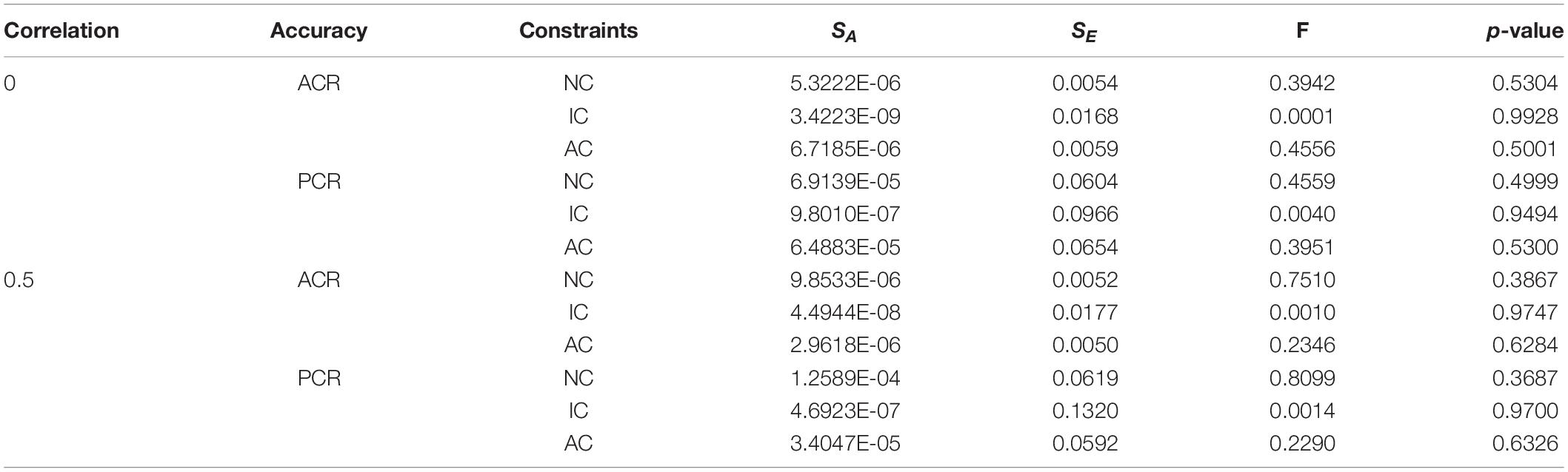
Table 1. Single factor analysis of variance for simplified and non-simplified constraints under the DINA model.
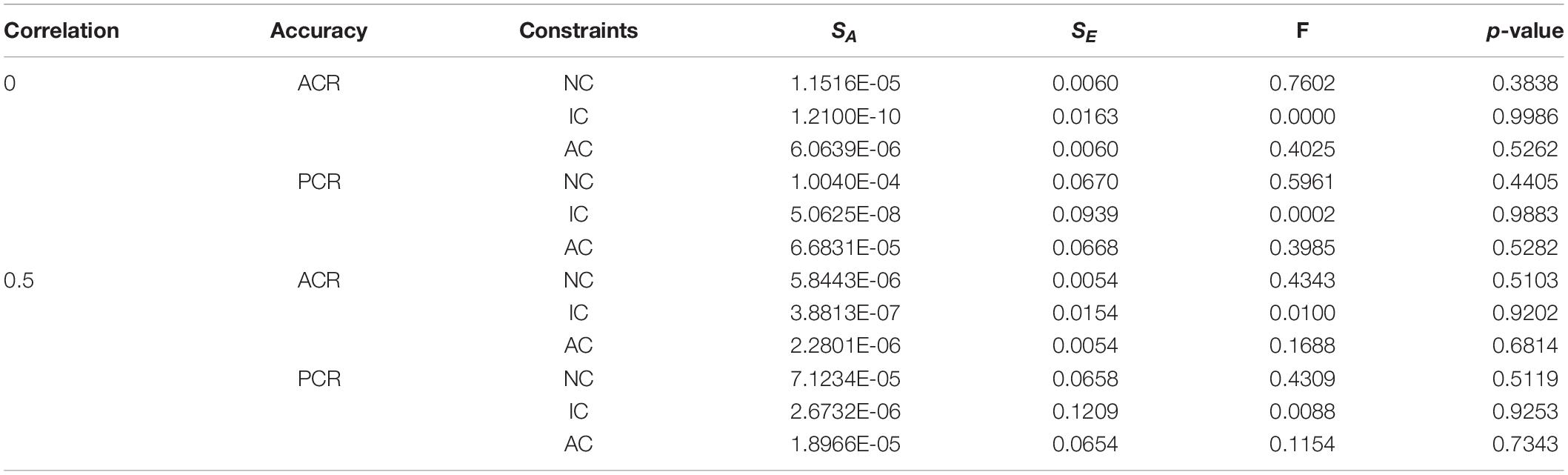
Table 2. Single factor analysis of variance for simplified and non-simplified constraints under the DINO model.

Table 3. Single factor analysis of variance for simplified and non-simplified constraints under the R-RUM model.
Tables 4–6 respectively give a detailed comparison of simplified and non-simplified constraints in terms of ACR and PCR under each condition of the DINA model, the DINO model and the R-RUM. The sixth column of the tables indicates that the accuracy rate of simplified constraints higher than the accuracy rate of non-simplified constraints.
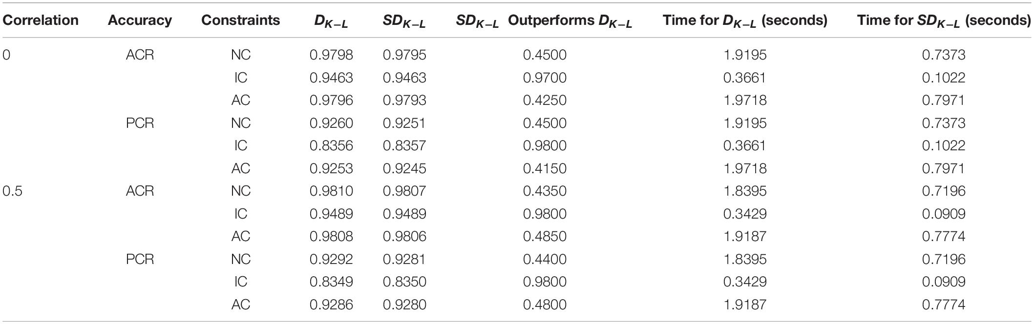
Table 4. Comparison of simplified and non-simplified constraints under the DINA model.
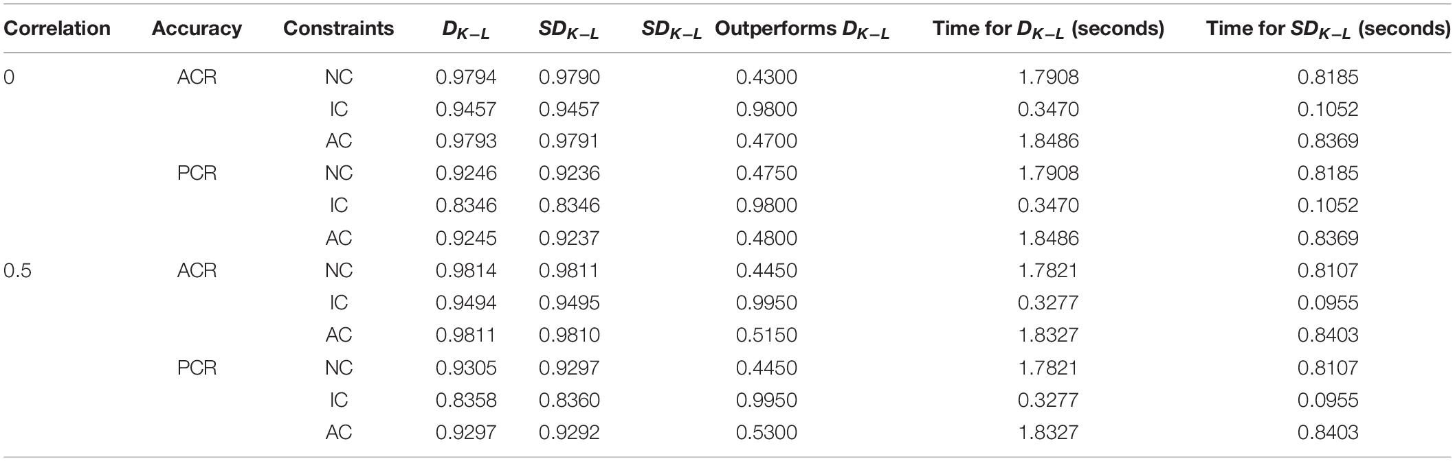
Table 5. Comparison of simplified and non-simplified constraints under the DINO model.
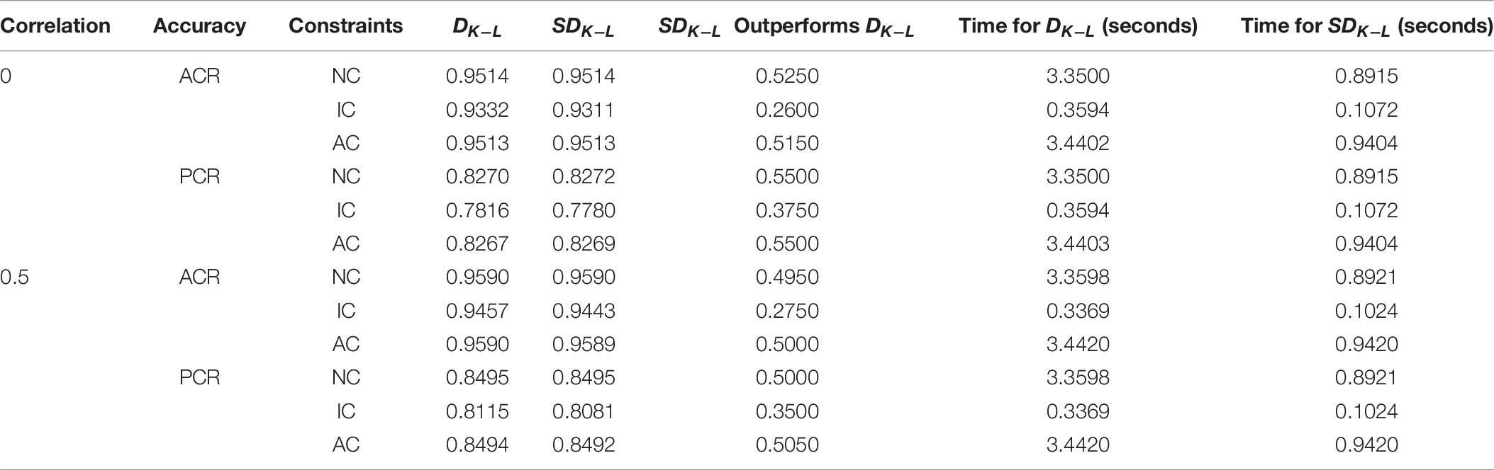
Table 6. Comparison of simplified and non-simplified constraints under the R-RUM model.
It can be seen from Table 4 that under the DINA model, when the MMD test assembly simplifies the constraints, the overall efficiency is less than 50% although the efficiency of the simplified constraints is higher than that of the non-simplified constraints. Therefore, the simplification of the distance matrix will indeed lose information. From the perspective of the overall mean, the loss of information has a relatively low impact on the efficiency of the test assembly. This conclusion is similar to the results of the one-way analysis of variance. In terms of average time consumption, simplifying the constraints will increase the operating efficiency by 2 to 4 times. Comparing with the information of lost by the simplified constraints, the improvement of the operating efficiency is considerable. Therefore, the simplified constraints on the distance matrix are feasible.
Tables 5, 6 shows that the efficiency of the simplified constraints is higher than that of the non-simplified constraints, the efficiency is more than 50% or close to 50% under the attribute constraints, but the overall situation is still lower than the non-simplified constraints and the difference is still small under the DINO model and R-RUM. In terms of time-consuming, the time-consuming for these two models is similar to that under the DINA model, but simplifying the constraints will still increase the operating efficiency by 2 to 4 times on average, so a similar conclusion can be obtained with the DINA model.
Study 2: Comparison Between Simplified MMD Method and CDI Method
Experimental Purpose
Study 1 has verified that the simplified constraints on the distance matrix is feasible, so how the new method itself compares with the famous method needs to be discussed further. In order to compare the simplified MMD test assembly method and the CDI method (Henson and Douglas, 2005), we performed the second simulation experiments by using the similar condition settings as the study of Henson and Douglas (2005). It should be noted that eight attributes were considered in the second simulation study for exploring the performance of the simplified MMD test assembly method under different conditions.
Experimental Steps
Conduct the simulation experiment as follows:
(1) According to the design of the first study, we simulated two groups of examinees, one of groups was used to calculate the prior distribution and the other was used for classification. The Q matrix and item parameters in the item bank and observed complete item response matrix of all possible attribute mastering patterns on all items in the item bank were simulated;
(2) Calculate the CDI and SDK−L of all items;
(3) Construct cognitive diagnostic test using the random way, the CDI method, or the simplified MMD method, according to the three strategies of no constraints, attribute constraints and item constraints;
(4) Take out the response matrix of all the items on the corresponding test according to the test items generated by the test assembly algorithms;
(5) Estimate the knowledge state of the examinees and calculate the PCR and ACR, according to the selected response matrix, and repeat experiments for a total of 200 times.
Experimental Results
Table 7 shows the average accuracy rate of each condition under measuring four attributes with the DINA model. In the table, CDI represents the CDI test assembly method, SDK−L is the simplified MMD test assembly method, and Random represents random test assembly. Analyzing the data in Table 7 shows that the new method has a higher improvement compared with the CDI method. In terms of the three constraints, the overall accuracy rate of the attribute constraints is slightly higher than the other two constraints, and the accuracy rate for the item constraints is the worst. Under the condition of item constraints, the ACR and PCR of CDI, MMD, and random test assembly method are lower than the other two constraints.
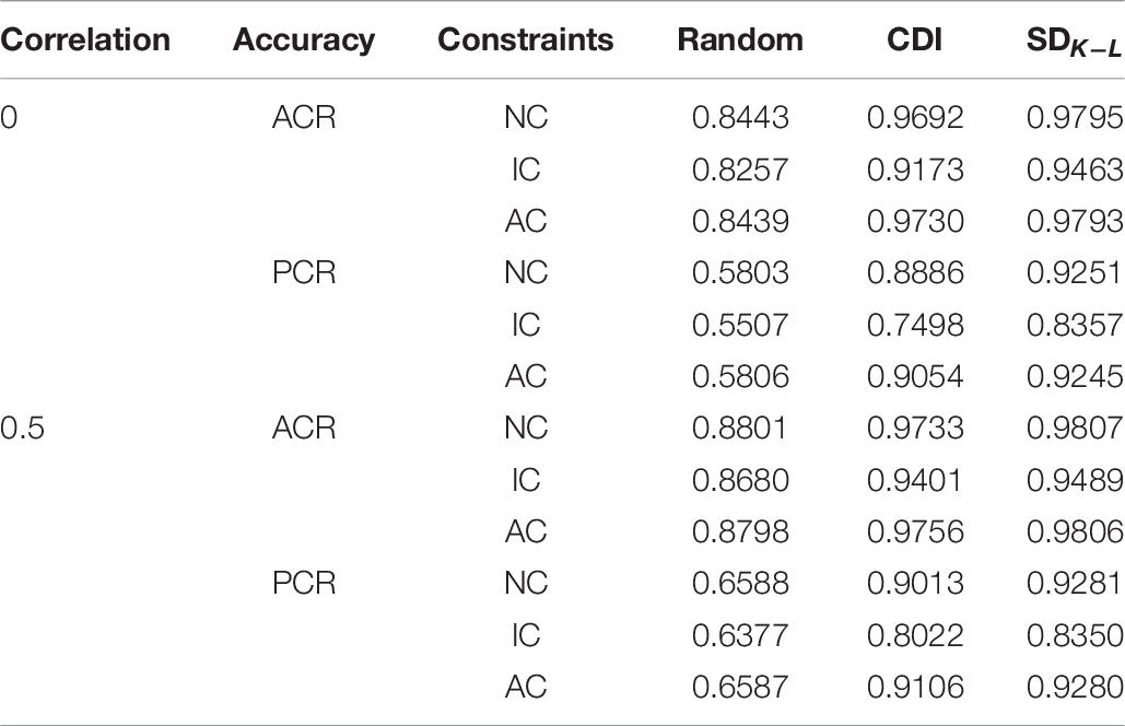
Table 7. The accuracy rate of each condition for four attributes under the DINA model.
Table 8 shows the comparison of the accuracy rate of each method when the number of attributes under the DINA model is four in the 200 repeats. Among them, the last column represents the proportion of MMD test assembly method with SDK−L distance as the class distance index more efficient than CDI in the 200 simulation repeats. The fourth or fifth column respectively represents the proportion of CDI test assembly method or MMD test assembly method with SDK−L distance more efficient than the random test assembly method across 200 repetitions.
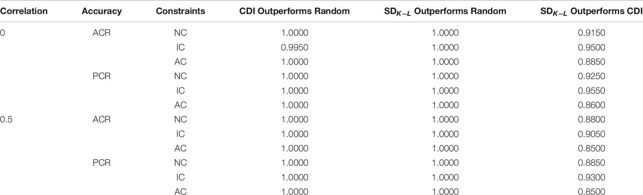
Table 8. Comparison of the accuracy rate of each method for four attributes under DINA model.
It can be seen from Table 8 that the MMD test assembly method with SDK−L distance as an index is stable under various conditions. In the existing conclusions, as the correlation increasing, the accuracy rate of the MMD test assembly method the CDI method based on SDK−L distance increases. Therefore, as the correlation increasing, the gap between the two methods will shrink. Thus, comparing with random test assembly, the average value of each method is greater than the random method. However, in the 200 simulation repeats, the CDI test assembly method is occasionally outperformed by the random test assembly method, which is similar to the simulation results of Henson and Douglas (2005).
On the whole, the result of CDI test assembly method is slightly different from that of Henson and Douglas (2005) in comparison with random test assembly method under measuring four attributes, because the random test assembly method itself is uncertain. In addition, the case that the accuracy rate of CDI test assembly method is lower than that of the random method is concentrated under the item constraints.
Table 9 shows the comparison of several test assembly methods for 200 repetitions under DINO model. From the data in Table 9, it can be seen that the MMD method is still superior to CDI method, and the MMD method with SDK−L distance as the distance index does not have the situation that the average accuracy rate is lower than CDI method.
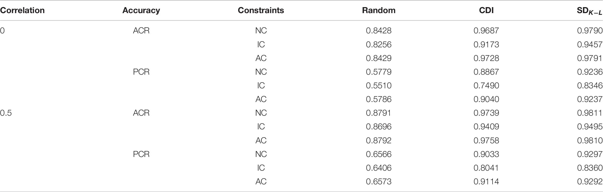
Table 9. Comparison of the accuracy rate of each method for four attributes under DINO model.
Table 10 shows the comparison of the accuracy rate of each method when the number of attributes is four across replications under the DINO model. It can be seen from Table 10, the MMD method with SDK−L distance as the distance index has slightly better accuracy rate than the CDI method under the condition of unconstrained and attribute constraints, respectively. However, the accuracy rate of the MMD test assembly method under the item constraints is better than under the other two constraints. In the existing conclusions, with the increase of correlation, the accuracy rate of MMD test assembly method with SDK−L distance as the index decreased while that of the CDI method increased. Therefore, with the increase of correlation, the gap between the two methods narrowed.
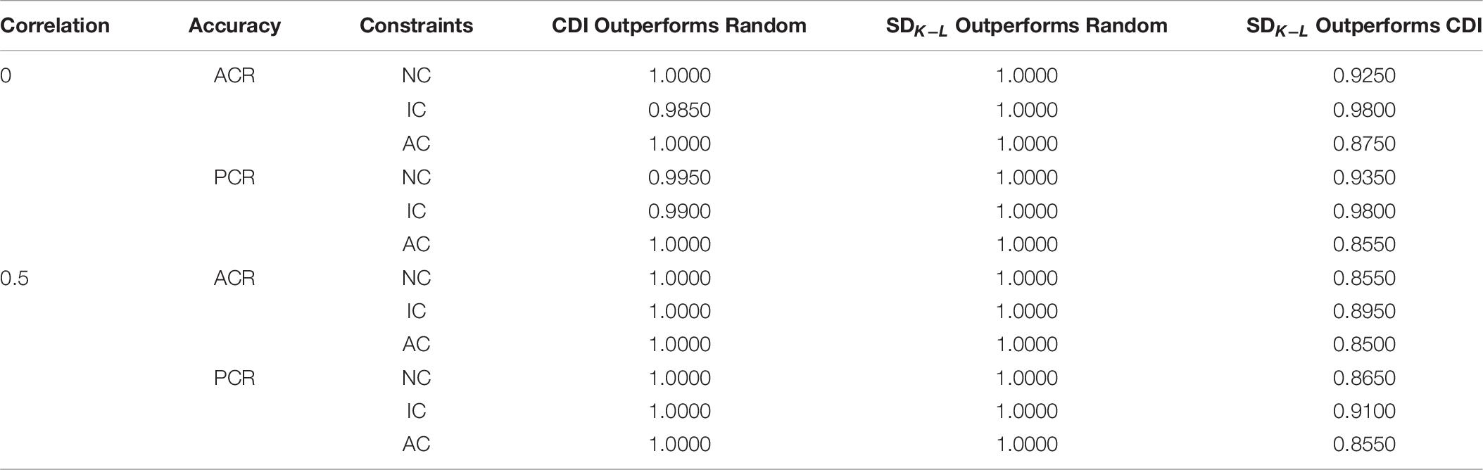
Table 10. Comparison of the accuracy rate of each method for four attributes under the DINO model.
Table 11 shows the comparison of several test assembly methods for the 200 repetitions under the R-RUM. Like the DINA and DINO model, the performance of MMD test assembly method based on SDK−L distance is better than the other two methods, and the performance is almost the same under the condition of both no constraints and attribute constraints.

Table 11. Comparison of the accuracy rate of each method for four attributes under R-RUM model.
Table 12 shows the comparison of the accuracy rate of each method when the number of attributes is four across replications under the R-RUM. It can be seen from Table 12 that in the 200 simulation replications, the MMD test assembly method based on SDK−L distance is better than the CDI test assembly method in every case, and its performance on R-RUM is also better than that of DINO model under the condition of both no constraints and attribute constraints.
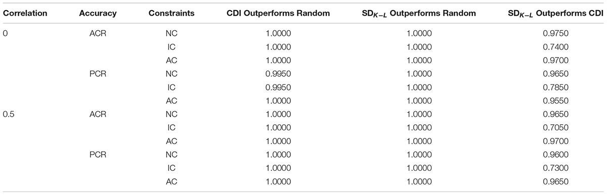
Table 12. Comparison of the accuracy rate of each method for four attributes under the R-RUM model.
Tables 13–18 show accuracy rates and comparison results for eight attributes. The results of eight attributes are similar to that of four attributes. On the whole, the new method is better than the CDI test assembly method and the random assembly method under the DINA model, the DINO model and the R-RUM. Furthermore, the new method has a greater advantage over the CDI method in terms of the PCR. Under the three models, the PCR of the MMD test assembly method based on SDK−L distance is higher than that of the CDI test assembly method, but the ACR of the MMD test assembly method is slightly lower than the CDI test assembly method. It means that the higher the averaged ACR, the PCR is not necessarily higher. For example, the ACRs for two attributes are 0.1 and 0.9 or 0.4 and 0.4. Although the average of ACR for these two cases are 0.5 and 0.4, the former case has the PCR of 0.09, while the latter case has the PCR of 0.16, if the correct classification rates for two attributes are independent.

Table 13. The accuracy rate of each condition for eight attributes under the DINA model.
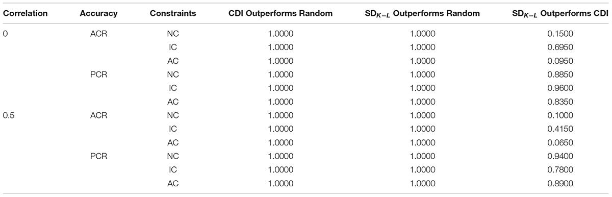
Table 14. Comparison of the accuracy rate of each method for eight attributes under the DINA model.
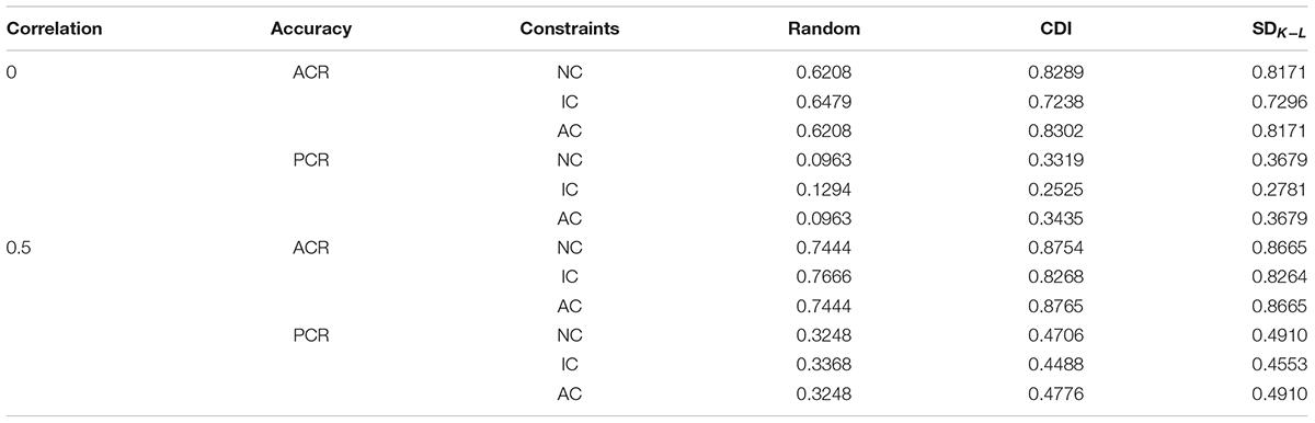
Table 15. The accuracy rate of each condition for eight attributes under the DINO model.
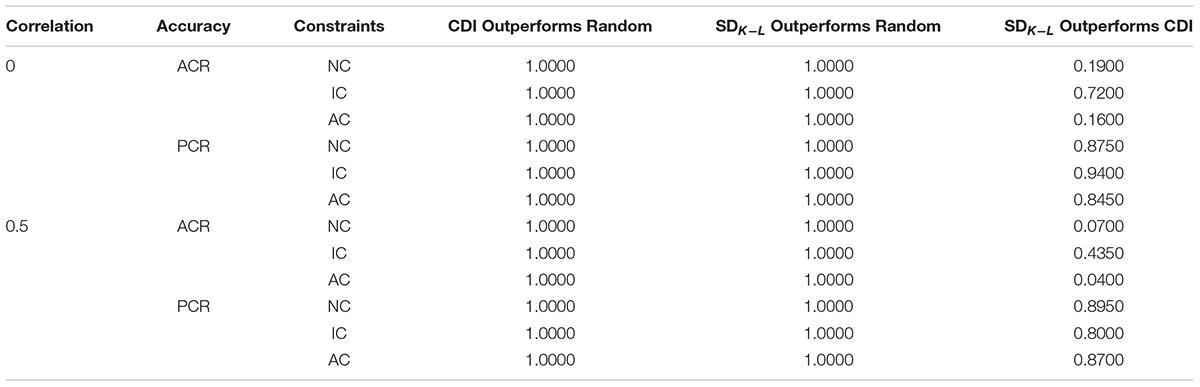
Table 16. Comparison of the accuracy rate of each method for eight attributes under the DINO model.
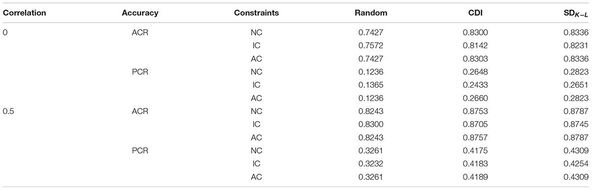
Table 17. The accuracy rate of each condition for eight attributes under the R-RUM model.
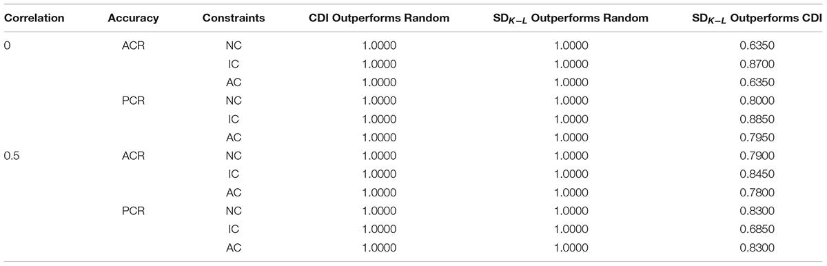
Table 18. Comparison of the accuracy rate of each method for eight attributes under the R-RUM model.
Discussion
Simulation results show that the MMD test assembly method with the simplified constraints has similar performance to the new method with the full constraints under four attributes, and the new simplified method performs better than the CDI method for four and eight attributes in term of the PCR. The MMD test assembly method with the full constraints suffers a large computational burden due to the optimization problem of complex constraints, but it is fast and performs relatively well when the number of attributes is four. In order to simplify computation, the MMD test assembly method with the simplified constraints can simplify computation effectively and is suitable for a larger number of attributes (i.e., eight attributes). We also found that when the number of measured attributes increases, the advantages in PCR for the MMD method are still obvious, while its performance in ACR tends to be average. This is related to the characteristics of the MMD and CDI-based test assembly methods: the CDI test assembly method pays attention to the local information, while the MMD focuses on the global information. When the ratio of test length to attribute number is large, the MMD test assembly method has enough room to play and select enough high-quality tests to obtain sufficient overall information, in order to make up for the lack of local information. So, the MMD test assembly method has obvious advantages at this condition.
We found that there is a considerably worse performance for item constraints compared to attribute constraints, which is consistent of results of Henson and Douglas (2005). The possible explanations are as follows: First, we think this may be related to the concept of statistical identification that is receiving a lot of attention lately for the case of CDMs. Specifically, for the DINA model, two identity matrices in the Q matrix and an additional third item per attribute would be required (e.g., Chen et al., 2015; Xu and Shang, 2018). This would be never satisfied in the item constraint condition. Second, because the item constraints required only 4 items measured one attribute, the Q-matrix is not complete if all columns of the K × K identity matrix are not contained in the Q-matrix. A simple example of a complete Q-matrix is the K × K identity matrix I (Chiu et al., 2009; Cai et al., 2018). Third, item-level expected classification accuracy of attributes for 16 items measured two or three attributes in item constraint condition is often lower than that for items measured only one attribute (Wang et al., 2019).
Test constraints in this study are still rough, since it is only a repetition of Henson and Douglas (2005) experiments. The performance of each method under other constraints needs to be studied. The MMD test assembly method with SDK−L distance as the index is superior to CDI test assembly method in performance, but the combination of this test assembly idea and other distance indexes is worth discussing. This study does not consider the relationship between the number of measured attributes and the length of tests, the influence of the ratio of the test length and number of attributes on the MMD test assembly method, how about the specific relationship between them is, and how to specify item constraints and attribute constraints when the length of tests is different, all of above will need a further investigation.
As in the study of Henson and Douglas (2005), the larger sample in our study was only employed to obtain correct classification rates more stability with simulated item parameters. We have not considered the impact of item banks calibrated by using larger or smaller sample sizes on the performance of test construction methods. As the reviewer motioned, it is true that larger sample sizes are likely to be used to calibrate item banks (e.g., Liu et al., 2013; George and Robitzsch, 2014), while the review of available empirical studies indicates that sample sizes in cognitive diagnosis tend to be much smaller (Sessoms and Henson, 2018). It would be an interesting question to justify whether a difference in performance is expected from the CDI and SDK−L methods for item banks calibrated from different sample sizes. One limitation of this study is that three simple CDMs (the DINA model, the DINO model, and the R-RUM) were considered in the simulation study. If we have a large sample size to calibrate an item bank, we believe that the results can be generalized to a more general model, such as the G-DINA model (de la Torre, 2011), or a combination of reduced models (Ravand, 2016; Sorrel et al., 2017; de la Torre et al., 2018).
Data Availability Statement
The raw data supporting the conclusions of this article will be made available by the authors, without undue reservation.
Author Contributions
WW and LS designed the study and wrote the manuscript. JZ, YT, and PG drafted and revised the manuscript. WW and PG conducted the simulation study. All authors contributed to the article and approved the submitted version.
Funding
This research was partially supported by the National Natural Science Foundation of China (Grant No. 62067005), the Social Science Foundation of Jiangxi (Grant No. 17JY10), the Project of Teaching Reform of Jiangxi Normal University (Grant No. JXSDJG1848), and the grant (Grant No. CTI2019B10) from the Chinese Testing International Co., Ltd.
Conflict of Interest
The authors declare that the research was conducted in the absence of any commercial or financial relationships that could be construed as a potential conflict of interest.
References
Cai, Y., Tu, D., and Ding, S. (2018). Theorems and methods of a complete Q matrix with attribute hierarchies under restricted q-matrix design. Front. Psychol. 9:1413. doi: 10.3389/fpsyg.2018.01413
Chang, H.-H., and Ying, Z. (1996). A global information approach to computerized adaptive testing. Appl. Psychol. Measurem. 20, 213–229. doi: 10.1177/014662169602000303
Chen, Y., Liu, J., Xu, G., and Ying, Z. (2015). Statistical analysis of Q-matrix based diagnostic classification models. J. Am. Statist. Assoc. 110, 850–866. doi: 10.1080/01621459.2014.934827
Chiu, C.-Y., Douglas, J. A., and Li, X. (2009). Cluster analysis for cognitive diagnosis: theory and applications. Psychometrika 74, 633–665. doi: 10.1007/s11336-009-9125-0
Clark, I. (2013). Efficacy of Formative Classroom Assessments in Theory and Practice. Doctoral dissertation University of Washington: Seattle, WA.
Cover T. M. and Thomas J. A. (ed.). (2006). Elements of Information Theory, 2nd Edn. Hoboken, NJ: John Wiley & Sons, Inc.
de la Torre, J., van der Ark, L. A., and Rossi, G. (2018). Analysis of clinical data from a cognitive diagnosis modeling framework. Measurement Eval. Counsel. Dev. 51, 281–296. doi: 10.1080/07481756.2017.1327286
de la Torre, J. (2011). The generalized DINA model framework. Psychometrika 76, 179–199. doi: 10.1007/s11336-011-9207-7
Debeer, D., Van Rijn, P. W., and Ali, U. S. (2020). Multidimensional test assembly using mixed-integer linear programming: an application of Kullback-Leibler information. Appl. Psychol. Measurement 44, 17–32. doi: 10.1177/0146621619827586
Finkelman, M., Kim, W., and Roussos, L. A. (2009). Automated test assembly for cognitive diagnosis models using a genetic algorithm. J. Educ. Measurement 46, 273–292. doi: 10.1111/j.1745-3984.2009.00081.x
George, A. C., and Robitzsch, A. (2014). Multiple group cognitive diagnosis models, with an emphasis on differential item functioning. Psychol. Test Assessm. Model. 56, 405–432.
Guo, L., Yang, J., and Song, N. (2020). Spectral clustering algorithm for cognitive diagnostic assessment. Front. Psychol. 11:944. doi: 10.3389/fpsyg.2020.00944
Hartz, S. (2002). A Bayesian Framework for the Unified Model for Assessing Cognitive Abilities: Blending Theory with Practicality, Unpublished doctoral dissertation University of Illinois at Urbana-Champaign: Champaign, IL.
Henson, R., and Douglas, J. (2005). Test construction for cognitive diagnosis. Appl. Psychol. Measurement 29, 262–277. doi: 10.1177/0146621604272623
Henson, R., Roussos, L., Douglas, J., and He, X. (2008). Cognitive diagnostic attribute-level discrimination indices. Appl. Psychol. Measurement 32, 275–288. doi: 10.1177/0146621607302478
Hsu, C. L., Jin, K. Y., and Chiu, M. M. (2020). Cognitive diagnostic models for random guessing behaviors. Front. Psychol. 11:570365. doi: 10.3389/fpsyg.2020.570365
Junker, B. W., and Sijtsma, K. (2001). Cognitive assessment models with few assumptions, and connections with nonparametric item response theory. Appl. Psychol. Measurement 25, 258–272. doi: 10.1177/01466210122032064
Kantor, I., Robineau, J. L., Bütün, H., and Maréchal, F. (2020). A mixed-integer linear programming formulation for optimizing multi-scale material and energy integration. Front. Energy Res. 8:49. doi: 10.3389/fenrg.2020.00049
Kuo, B.-C., Pai, H.-S., and de la Torre, J. (2016). Modified cognitive diagnostic index and modified attribute-level discrimination index for test construction. Appl. Psychol. Measurement 40, 315–330. doi: 10.1177/0146621616638643
Liu, H. Y., You, X. F., Wang, W. Y., Ding, S. L., and Chang, H. H. (2013). The development of computerized adaptive testing with cognitive diagnosis for an English achievement test in China. J. Classif. 30, 152–172. doi: 10.1007/s00357-013-9128-5
Madigan, D., and Almond, R. (1995). “On test selection strategies for belief networks,” in Learning From Data: AI and Statistics V, eds D. Fisher and H.-J. Lenz (New York, NY: Springer-Verlag), 89–98. doi: 10.1007/978-1-4612-2404-4_9
Mao, X. Z. (2014). The attribute mastery probability cognitive diagnostic model. J. Sichuan Normal University 37, 373–443.
Rao, C. R. (1962). Efficient estimates and optimum inference procedures in large samples. J. R. Statist. Soc. Series B 24, 46–72. doi: 10.1111/j.2517-6161.1962.tb00436.x
Ravand, H. (2016). Application of a cognitive diagnostic model to a high-stakes reading comprehension test. J. Psychoeduc. Assess. 34, 782–799. doi: 10.1177/0734282915623053
Sessoms, J., and Henson, R. A. (2018). Applications of diagnostic classification models: a literature review and critical commentary. Measurement: Interdiscipl. Res. Perspect. 16, 1–17. doi: 10.1080/15366367.2018.1435104
Sia, C. J. L., and Lim, C. S. (2018). “Cognitive diagnostic assessment: an alternative mode of assessment for learning,” in Classroom Assessment in Mathematics. ICME-13 Monographs, eds D. Thompson, M. Burton, A. Cusi, and D. Wright (Cham: Springer).
Sorrel, M. A., Abad, F. J., Olea, J., de la Torre, J., and Barrada, J. R. (2017). Inferential item-fit evaluation in cognitive diagnosis modeling. Appl. Psychol. Measurement 41, 614–631. doi: 10.1177/0146621617707510
Tang, F., and Zhan, P. D. (2020). The development of an instrument for longitudinal learning diagnosis of rational number operations based on parallel tests. 11:2246. doi: 10.3389/fpsyg.2020.02246
Tatsouka, C., and Ferguson, T. (2003). Sequential classification on partially ordered sets. J. R. Statist. Soc.: Series B 65, 143–158. doi: 10.1111/1467-9868.00377
Templin, J. L., and Henson, R. A. (2006). Measurement of psychological disorders using cognitive diagnosis models. Psychol. Methods 11, 287–305. doi: 10.1037/1082-989x.11.3.287
Wang, W. Y., Gao, P., Song, L. H., and Wang, T. (2020). The improved exploratory method of Q-matrix specification with noise preprocessing. J. Jiangxi Normal University 44, 136–141.
Wang, W. Y., Song, L. H., Chen, P., and Ding, S. L. (2019). An item-level expected classification accuracy and its applications in cognitive diagnostic assessment. J. Educ. Measurement 56, 51–75. doi: 10.1111/jedm.12200
Xu, G., and Shang, Z. (2018). Identifying latent structures in restricted latent class models. J. Am. Statist. Assoc. 113, 1284–1295. doi: 10.1080/01621459.2017.1340889
Keywords: cognitive diagnosis, cognitive diagnostic model information index, cluster analysis, mixed-integer linear programming, inter-class distance, correct classification rate
Citation: Wang W, Zheng J, Song L, Tu Y and Gao P (2021) Test Assembly for Cognitive Diagnosis Using Mixed-Integer Linear Programming. Front. Psychol. 12:623077. doi: 10.3389/fpsyg.2021.623077
Received: 29 October 2020; Accepted: 11 January 2021;
Published: 02 February 2021.
Edited by:
Liu Yanlou, Qufu Normal University, ChinaReviewed by:
Chunhua Kang, Zhejiang Normal University, ChinaMiguel A. Sorrel, Autonomous University of Madrid, Spain
Copyright © 2021 Wang, Zheng, Song, Tu and Gao. This is an open-access article distributed under the terms of the Creative Commons Attribution License (CC BY). The use, distribution or reproduction in other forums is permitted, provided the original author(s) and the copyright owner(s) are credited and that the original publication in this journal is cited, in accordance with accepted academic practice. No use, distribution or reproduction is permitted which does not comply with these terms.
*Correspondence: Wenyi Wang, wenyiwang@jxnu.edu.cn; Lihong Song, viviansong1981@163.com