Definable Conditionals

Abstract

The variably strict analysis of conditionals does not only largely dominate the philosophical literature, since its invention by Stalnaker and Lewis, it also found its way into linguistics and psychology. Yet, the shortcomings of Lewis–Stalnaker’s account initiated a plethora of modifications, such as non-vacuist conditionals, presuppositional indicatives, perfect conditionals, or other conditional constructions, for example: reason relations, difference-making conditionals, counterfactual dependency, or probabilistic relevance. Many of these new connectives can be treated as strengthened or weakened conditionals. They are definable conditionals. This article develops a technique to infer the logic for such definable conditionals from the known logic of the underlying defining conditional. The technique is applied to central examples. The results show that a large part of the zoo of conditionals arises from a basic conditional—a constant nucleus of the different contextual and conceptual variations of variably strict conditionals.

1 Introduction

Conditionals are notoriously difficult to analyse. Conditionals are natural language sentences of the form ‘if A then C’, where A is the antecedent and C the consequent. A standard account has however emerged, the so-called possible worlds account (Stalnaker 1968; Lewis 1973b). According to this account, a conditional $A> C$ is true in the actual world (roughly) if and only if the closest A-worlds are C-worlds.¹ However, recent reflections suggest that the defining clause needs to be strengthened by additional conditions. What these conditions are is not settled. Different approaches argue for different conditions (Krzyżanowska et al. 2013; Spohn 2015; Skovgaard-Olsen 2016; Raidl 2019; Rott 2019; Crupi and Iacona 2019). Some of these logics are not worked out yet, or only for specific semantics. To compare them, we need to know how the logic changes with the semantics, and vice versa. The article develops a technique to answer these questions.

The general problem is this: Take a strengthened conditional of the form

• $\varphi {{\,\mathrm{\vartriangleright }\,}}\psi$ in the actual world iff closest $\varphi$-worlds are $\psi$-worlds and X.

Suppose that X is also formulated in terms of closeness. The conditional $\varphi {{\,\mathrm{\vartriangleright }\,}}\psi$ can then be rephrased in the language for >, namely as $(\varphi > \psi ) \wedge \chi$, where $\chi$ expresses the semantic condition X. The following question arises:

• Can we use known completeness results for > to obtain completeness results for ${{\,\mathrm{\vartriangleright }\,}}$?

The answer is yes and the paper provides a general method. The method also applies to weakened conditionals, where in the defining clause one replaces ‘and’ by ‘or’ and thus $\wedge$ by $\vee$, and more generally to definable conditionals. The idea goes as follows: Redefine > in terms of ${{\,\mathrm{\vartriangleright }\,}}$. This yields a formula $\alpha$ in the language for ${{\,\mathrm{\vartriangleright }\,}}$. We can use this backtranslation to translate axioms for > into axioms for ${{\,\mathrm{\vartriangleright }\,}}$. The backtranslation is a looking glass showing a distorted picture of the logic for >. This picture is a logic for ${{\,\mathrm{\vartriangleright }\,}}$.

The plan of the paper is as follows. Section 2 sets the stage with a flexible framework for conditionals. Section 3 introduces the translation between conditional languages. Section 4 defines semantic conditions for a translation to be well behaved. Section 5 introduces the backtranslation and axiomatic conditions for it to be well behaved. Section 6 develops the technique of transferring soundness, completeness and correspondence results. Section 7 applies this to the sufficient reason relation. Section 8 shows how to chain the transfer of results, illustrated by the necessary reason relation. Section 9 applies the method to alternative semantics, exemplified by ranking and belief revision semantics. The Conclusion (Sect. 10) comments on further applications.

2 Basic Conditional Logic

This section rehearses some known conditional logics and introduces the semantics used for the basic conditional >. The results considered here are known or analogue to famous results in modal logics, and thus proofs are omitted.

The alphabet of our basic conditional language is based on a fixed set of propositional variables ${{\,\mathrm{\text{ Var }}\,}}$, classical connectives, $\lnot , \wedge , \vee$ and $\rightarrow$ (the material conditional), and the basic conditional >, as well as the parenthesis ) and (. The set of formulas is defined inductively and is denoted ${{\,\mathrm{\mathcal {L}}\,}}_>$. In what follows $\top$ denotes any classical propositional tautology and $\bot = \lnot \top$. Let $\varGamma$ be an axiomatic system in ${{\,\mathrm{\mathcal {L}}\,}}_>$, given by a set of axioms and a set of inference rules. We write $\vdash _{_{\varGamma }} \varphi$ iff there is a proof of $\varphi$ in $\varGamma$, defined as usual.

Possible rules of conditional logic are:²

Some well known axioms are:

• $\varphi > \top$ (${{\mathsf {CN}}}$, –)

• $(\varphi> \psi ) \rightarrow (\varphi > (\psi \vee \chi ))$ (${{\mathsf {Cm}}}$, RW)

• $((\varphi> \psi ) \wedge (\varphi> \chi )) \rightarrow (\varphi > (\psi \wedge \chi ))$ (${{\mathsf {CC}}}$, AND)

• $\varphi > \varphi$ (${{\mathsf {ID}}}$, Refl)

• $((\varphi> \chi ) \wedge (\psi> \chi )) \rightarrow ((\varphi \vee \psi ) > \chi )$ (${{\mathsf {CA}}}$, OR)

• $((\varphi> \chi ) \wedge (\varphi> \psi )) \rightarrow ((\varphi \wedge \psi ) > \chi )$ (${{\mathsf {CMon}}}$, CM)

• $((\varphi> \chi ) \wedge \lnot (\varphi> \lnot \psi )) \rightarrow ((\varphi \wedge \psi ) > \chi )$ (${{\mathsf {CV}}}$, RM)

Throughout the article, I use the left notation—the ${{\mathsf {X}}}$ appearing in (${{\mathsf {X}}}$, Y). The rule ${{\mathsf {RCEC}}}$ combined with the axiom ${{\mathsf {Cm}}}$ is equivalent to the rule:

Furthermore, given ${{\mathsf {Cm}}}$ and the axiom ${{\mathsf {ID}}}$, the axiom ${{\mathsf {CN}}}$ is redundant.

We say that ${{\mathsf {L}}}\subseteq {{\,\mathrm{\mathcal {L}}\,}}_>$ is a conditional logic iff it contains all substitution instances of propositional tautologies (${{\mathsf {PT}}}$) and is closed under Modus Ponens for $\rightarrow$ (${{\mathsf {MoPo}}}$). We denote ${{\mathsf {L}}}+ {{\mathsf {X}}}_1 + \ldots + {{\mathsf {X}}}_n$ the smallest conditional logic closed under the rules of ${{\mathsf {L}}}$, containing the axioms of ${{\mathsf {L}}}$, as well as the axioms ${{\mathsf {X}}}_1, \ldots , {{\mathsf {X}}}_n$. As an example, the smallest classical conditional logic is ${{\mathsf {CE}}} = {{\mathsf {RCEA}}} + {{\mathsf {RCEC}}} + {{\mathsf {MoPo}}} + {{\mathsf {PT}}}$. The smallest normal conditional logic is ${{\mathsf {CK}}} = {{\mathsf {CE}}} + {{\mathsf {Cm}}} + {{\mathsf {CN}}} + {{\mathsf {CC}}}$.

In what follows, $f:X {{\,\mathrm{\longrightarrow }\,}}Y$ indicates that f is a total function from X to Y. To model the logic ${{\mathsf {CE}}}$ and extensions, I adopt a flexible semantics introduced by Chellas (1975):

Definition 1

Let W be a non-empty set. ${{\,\mathrm{\mathfrak {F}}\,}}= {{\,\mathrm{\langle }\,}}W, F{{\,\mathrm{\rangle }\,}}$ is a minimal frame iff $F:(W \times \wp (W)) {{\,\mathrm{\longrightarrow }\,}}\wp (\wp (W))$. ${{\,\mathrm{\mathfrak {M}}\,}}= {{\,\mathrm{\langle }\,}}W, F, V{{\,\mathrm{\rangle }\,}}$ is a minimal model for ${{\,\mathrm{\mathcal {L}}\,}}_>$ iff ${{\,\mathrm{\langle }\,}}W, F{{\,\mathrm{\rangle }\,}}$ is a minimal frame and $V:{{\,\mathrm{\text{ Var }}\,}}{{\,\mathrm{\longrightarrow }\,}}\wp (W)$.

The points in W are commonly called worlds. Subsets of W are commonly called propositions. The neighbourhood selection function F associates to every world and every proposition A a set of propositions F(w, A). This can be interpreted as the A-neighbourhood of w. One may think of it as a set of options triggered by supposing A, or as the set of believed propositions after supposing, or revising by A. This semantics allows to model much weaker logics than the Lewis–Stalnaker account.

Definition 2

Truth in a minimal model ${{\,\mathrm{\mathfrak {M}}\,}}$ for ${{\,\mathrm{\mathcal {L}}\,}}_>$ is denoted and defined as follows:

• 1. iff $w \in V(p)$ when $p \in {{\,\mathrm{\text{ Var }}\,}}$,

• 2. iff ,

• 3. iff and ,

• 4. iff or ,

• 5. iff or ,

• 6. iff .

The sets are co-inductively defined.

The truth clauses for propositional variables and the standard connectives are known from modal logic. The truth clause for the conditional says this: the conditional $\varphi > \psi$ is true in w if and only if the set of $\psi$-worlds is in the $\varphi$-neighbourhood, or the proposition $\psi$ is an option when supposing $\varphi$, or the proposition $\psi$ is believed after revising by $\varphi$.

I adopt standard notation and write: iff for all . iff for all models ${{\,\mathrm{\mathfrak {M}}\,}}$ over ${{\,\mathrm{\mathfrak {F}}\,}}$, . And for C a class (of models or frames): iff for all $X \in C$, . When the model ${{\,\mathrm{\mathfrak {M}}\,}}$ is clear from the context, I drop upper indices, writing instead of and $[\varphi ]{{\,\mathrm{_{\scriptscriptstyle >}}\,}}$ instead of $[\varphi ]{{\,\mathrm{^{\scriptscriptstyle {{\,\mathrm{\mathfrak {M}}\,}}}_{\scriptscriptstyle >}}\,}}$. When the language is clear, I drop lower indices.

The following was proven by a canonical model construction (Chellas 1975):

Theorem 1

${{\mathsf {CE}}}$ is sound and complete for the class of minimal frames (models) M, i.e., $\vdash _{_{{{\mathsf {CE}}}}} \alpha$ iff for all $\alpha \in {{\,\mathrm{\mathcal {L}}\,}}_>$.

For minimal frames, we can translate axioms into properties of the neighbourhood selection function: for $\varphi$ becoming $A = [\varphi ]$, $\psi$ becoming B and $\chi$ becoming C, $\varphi > \psi$ becomes $B \in F(w, A)$. Inner logical operators ($\top , \bot , \lnot , \wedge , \vee , \rightarrow$ in the scope of >) are translated algebraically: $\top$ becomes W, $\bot$ becomes $\emptyset$, $\lnot \varphi$ becomes $\overline{A}=W \setminus A$, $\wedge$ becomes $\cap$, $\vee$ becomes $\cup$ and $\varphi \rightarrow \psi$ becomes $\overline{A} \cup B$. Outer logical operators are translated in the natural language. For ${{\mathsf {X}}}$ a conditional axiom, we denote ${{\mathsf {X}}}^F$ or just (x) its corresponding minimal frame property, obtained by the mentioned transformation. The axiom schemes introduced above, have the following corresponding frame properties, quantified over all $w \in W$ and all subsets A, B, C of W:

$$\begin{aligned} \begin{array}{lr} W \in F(w, A) &{} ({{\mathsf {CN}}}^F, \, \hbox {cn})\\ B \in F(w, A) \hbox { implies } B \cup C \in F(w, A) &{} ({{\mathsf {Cm}}}^F, \,\hbox { cm})\\ B \in F(w, A) \text { and } C \in F(w, A) \text { imply } B \cap C \in F(w, A) &{} ({{\mathsf {CC}}}^F,\, \hbox { cc})\\ A \in F(w,A) &{} ({{\mathsf {ID}}}^F,\hbox { id})\\ C \in F(w, A)\hbox { and }C \in F(w, B) \text { imply } C \in F(w, A \cup B) &{} ({{\mathsf {CA}}}^F,\,\hbox { ca})\\ C \in F(w, A)\hbox { and }B \in F(w, A) \text { imply } C \in F(w, A \cap B) &{} ({{\mathsf {CMon}}}^F,\,\hbox { cmon})\\ C \in F(w, A)\hbox { and }\overline{B} \notin F(w, A) \text { imply } C \in F(w, A \cap B) &{} ({{\mathsf {CV}}}^F,\,\hbox { cv})\\ \end{array} \end{aligned}$$

“Correspondence” has a precise meaning—the same as in the correspondence theory for modal logic. Let ${{\mathsf {X}}}$ be an axiom scheme. We write $w {{\,\mathrm{\vDash }\,}}{{\mathsf {X}}}$ iff $w {{\,\mathrm{\vDash }\,}}\varphi$ for all $\varphi \in {{\mathsf {X}}}$. This lifts truth from formulas to axiom schemes. Similarly for models, frames and classes. The correspondence theory for minimal frames says that an axiom scheme is valid in a frame if and only if the frame has the property corresponding to the axiom scheme:

Theorem 2

For ${{\,\mathrm{\mathfrak {F}}\,}}$ a minimal frame, iff ${{\,\mathrm{\mathfrak {F}}\,}}$ satisfies ${{\mathsf {X}}}^F$.

From this and Theorem 1, completeness results for extensions of ${{\mathsf {CE}}}$ follow:

Theorem 3

Let ${{\mathsf {X}}}_1, \ldots , {{\mathsf {X}}}_n$ be axiom schemes (from our list) and ${{\mathsf {X}}}^F_1, \ldots , {{\mathsf {X}}}^F_n$ the corresponding frame properties. Then the logic ${{\mathsf {CE}}} + {{\mathsf {X}}}_1 + \ldots + {{\mathsf {X}}}_n$ is sound and complete for the class C of those minimal frames (or models) which satisfy ${{\mathsf {X}}}^F_1, \ldots , {{\mathsf {X}}}^F_n$.

Proof

Soundness follows from Theorem 2. Completeness is proven by re-running Chellas’ canonical model construction for Theorem 1, noting that the canonical model ${{\,\mathrm{\mathfrak {M}}\,}}^{\varSigma }$ for $\varSigma = {{\mathsf {CE}}} + {{\mathsf {X}}}_1 + \ldots + {{\mathsf {X}}}_n$ has the properties ${{\mathsf {X}}}^F_1, \ldots , {{\mathsf {X}}}^F_n$. $\square$

For latter sections, we need axioms for the outer and inner modalities. The outer necessity is ${{\,\mathrm{\square }\,}}\alpha \equiv (\lnot \alpha > \bot )$ and the inner necessity is ${{\,\mathrm{\boxdot }\,}}\alpha \equiv (\top > \alpha )$. The outer possibility and inner possibility are defined as duals to ${{\,\mathrm{\square }\,}}$ and ${{\,\mathrm{\boxdot }\,}}$, as usual. The following are axioms for the inner and outer modalities, which I also reformulate in their modal form:

$$\begin{aligned} \begin{array}{llr} (\varphi> \psi ) \rightarrow (\top> (\lnot \varphi \vee \psi ))&{}(\varphi> \psi ) \rightarrow {{\,\mathrm{\boxdot }\,}}(\varphi \rightarrow \psi ) &{}({{\mathsf {INC}}})\\ ((\top> \psi ) \wedge \lnot (\top> \lnot \varphi )) \rightarrow (\varphi> \psi ) &{} ({{\,\mathrm{\boxdot }\,}}\psi \wedge {{\,\mathrm{\Diamond \cdot ~}\,}}\varphi ) \rightarrow (\varphi> \psi ) &{} ({{\mathsf {PRES}}})\\ (\varphi> \bot ) \rightarrow ((\varphi \wedge \psi )> \bot ) &{}{{\,\mathrm{\Diamond }\,}}(\varphi \wedge \psi ) \rightarrow {{\,\mathrm{\Diamond }\,}}\varphi &{} ({{\mathsf {M}}})\\ ((\varphi> \bot ) \wedge (\psi> \bot )) \rightarrow ((\varphi \vee \psi )> \bot ) &{} {{\,\mathrm{\Diamond }\,}}(\varphi \vee \psi ) \rightarrow ({{\,\mathrm{\Diamond }\,}}\varphi \vee {{\,\mathrm{\Diamond }\,}}\psi ) &{} ({{\mathsf {C}}})\\ \lnot (\top > \bot ) &{}\lnot {{\,\mathrm{\square }\,}}\bot &{} ({{\mathsf {P}}})\\ \end{array} \end{aligned}$$

Assume $\mathsf {CE+ RCM}$. Then ${{\mathsf {INC}}}$ follows from ${{\mathsf {CA}}}$, given ${{\mathsf {ID}}}$. It is known from belief revision as the postulate of Inclusion. ${{\mathsf {PRES}}}$ is an instance of ${{\mathsf {CV}}}$. It is known as the postulate of Preservation.³ In ${{\mathsf {CK}}}$, the inner necessity is a normal necessity. ${{\mathsf {M}}}$ follows from ${{\mathsf {CMon}}}$. It says that the outer necessity is monotone. ${{\mathsf {C}}}$ is an instance of ${{\mathsf {CA}}}$, it says that the outer necessity is closed under conjunction. The outer necessity is a normal necessity in ${{\mathsf {CE}}} + {{\mathsf {ID}}} + {{\mathsf {CMon}}} + {{\mathsf {CA}}}$. ${{\mathsf {P}}}$, known as probabilistic consistency, says that the outer and inner modality are consistent.

We will also use the following weakening of ${{\mathsf {CC}}}$:

• $(\varphi> \psi ) \rightarrow (\varphi > (\varphi \wedge \psi ))$ (${{\mathsf {WCC}}}$)

This axiom is redundant in the presence of ${{\mathsf {CC}}} + {{\mathsf {ID}}}$. Additionally, in a classical conditional logic with ${{\mathsf {Cm}}}$ and ${{\mathsf {WCC}}}$, the axioms ${{\mathsf {CN}}}$ and ${{\mathsf {ID}}}$ are equivalent. The frame properties for the new axioms should be clear, and Theorems 2 and 3 extend to these.

3 Translating

This section introduces the idea of translating between conditional languages. Translations are powerful cognitive tools. They allow us to understand another language. In logic, they also provide a powerful methodological tool, since by relating one language to another, they also link different semantics or logics. Modal logic is full of such translations. For example, the standard translation of modal formulas into first-order formulas, or Kripke’s translation of intuitionistic into modal logic. The first links Kripke models to relational structures and thereby builds a bridge between modal and classical worlds. Its methodological power lies in transferring results from first order logic to modal logic, for example compactness, the Löwenheim–Skolem property or recursive enumerability of validities. Similarly, Kripke’s translation makes us see intuitionism with modal and ultimately classical eyes. In brief, a translation is a lens through which we see the unknown in the shape of the known, it is also a conversion-machine which transfers known results to unknown domains. This is how we will use translations for conditionals.

Translating between conditional languages involves two languages, say ${{\,\mathrm{\mathcal {L}}\,}}_>$ and ${{\,\mathrm{\mathcal {L}}\,}}_{{{\,\mathrm{\vartriangleright }\,}}}$. Here, the language ${{\,\mathrm{\mathcal {L}}\,}}_{{{\,\mathrm{\vartriangleright }\,}}}$ is exactly like ${{\,\mathrm{\mathcal {L}}\,}}_>$, where ${{\,\mathrm{\vartriangleright }\,}}$ is a notational variant of >. The shared fragment of the two languages is the classical propositional language, denoted ${{\,\mathrm{\mathcal {L}}\,}}$. However, semantically ${{\,\mathrm{\vartriangleright }\,}}$ will be interpreted differently than >. I will provide several examples of such conditionals.

As a first toy example, consider the language ${{\,\mathrm{\mathcal {L}}\,}}_{>^C}$, where $>^C$ is to be interpreted as the complement conditional. The frames and models for ${{\,\mathrm{\mathcal {L}}\,}}_{>^C}$ are the same as for ${{\,\mathrm{\mathcal {L}}\,}}_>$. The truth clauses are not. In particular, the truth clause for $>^C$ differs from the truth clause for >. Truth in a minimal model ${{\,\mathrm{\mathfrak {M}}\,}}$ for the language ${{\,\mathrm{\mathcal {L}}\,}}_{>^C}$ is denoted . Since the truth clauses for propositional variables and classical connectives is defined as usual (as in ${{\,\mathrm{\mathcal {L}}\,}}_>$), I will not repeat them, and I use this short-cut throughout the article:

Example 1

The truth clause for the complement conditional is

$6_{C}$.:

iff $[\lnot \psi ]{{\,\mathrm{_{\scriptscriptstyle C}}\,}}\in F(w, [\lnot \varphi ]{{\,\mathrm{_{\scriptscriptstyle C}}\,}})$.

From the semantic clause one sees that if $>^C$ were in the language ${{\,\mathrm{\mathcal {L}}\,}}_>$, we could simply define $\varphi >^C \psi$ as $\lnot \varphi > \lnot \psi$. However, $>^C$ is not in the language ${{\,\mathrm{\mathcal {L}}\,}}_>$. Thus to state a relation between ${{\,\mathrm{\mathcal {L}}\,}}_>$ and ${{\,\mathrm{\mathcal {L}}\,}}_{>^C}$, we need other resources. This is the role of the translation between conditional languages.

Let $\theta$ be a formula of ${{\,\mathrm{\mathcal {L}}\,}}_>$ and p, q propositional variables. We write $\theta = \theta [p,q]$ iff $\theta$ has its propositional variables among $\{p, q\}$. That is, at least one of p and q must occur in $\theta$ and no other variable occurs in $\theta$. We write $\theta [p,q] \in {{\,\mathrm{\mathcal {L}}\,}}_>$ as an abbreviation for $\theta \in {{\,\mathrm{\mathcal {L}}\,}}_>, p,q \in {{\,\mathrm{\text{ Var }}\,}}$ and $\theta = \theta [p,q]$. Let $\varphi , \psi$ be formulas of ${{\,\mathrm{\mathcal {L}}\,}}_>$ and $\theta [p,q] \in {{\,\mathrm{\mathcal {L}}\,}}_>$, then we write $\theta [\varphi /p, \psi /q]$ for substituting simultaneously $\varphi$ for p and $\psi$ for q in $\theta$, defined as usual.

Definition 3

A translation is a total function $\circ :{{\,\mathrm{\mathcal {L}}\,}}_{{{\,\mathrm{\vartriangleright }\,}}} {{\,\mathrm{\longrightarrow }\,}}{{\,\mathrm{\mathcal {L}}\,}}_>$ such that

• 1. $p^{\circ }=p$, for $p \in {{\,\mathrm{\text{ Var }}\,}}$,

• 2. $(\lnot \varphi )^{\circ }=\lnot \varphi ^{\circ }$,

• 3. $(\varphi * \psi )^{\circ } = (\varphi ^{\circ } * \psi ^{\circ })$ for $* \in \{\wedge , \vee , \rightarrow \}$,

• 4. there is a formula $\theta [p, q] \in {{\,\mathrm{\mathcal {L}}\,}}_>$ such that for every $\varphi , \psi$ in ${{\,\mathrm{\mathcal {L}}\,}}_{{{\,\mathrm{\vartriangleright }\,}}}$, $(\varphi {{\,\mathrm{\vartriangleright }\,}}\psi )^{\circ } = \theta [\varphi ^{\circ }/p, \psi ^{\circ }/q]$.

A translation replaces formulas from ${{\,\mathrm{\mathcal {L}}\,}}_{{{\,\mathrm{\vartriangleright }\,}}}$ by formulas in ${{\,\mathrm{\mathcal {L}}\,}}_>$—as if we were translating English to Genglish where, say, we only replace some of the English words by German words. It is only the conditional which makes translating necessary—we are only replacing one particular English sentence form (the conditional) by a German one. This creates recursive echoes. Indeed, the fourth clause is the central one. It says that $\theta$ provides the form for the translate of $\varphi {{\,\mathrm{\vartriangleright }\,}}\psi$. Since the translate of classical connectives is fixed, it suffices to state the translate of the conditional, by providing $\theta$. We will say that the translation is induced from $(\varphi {{\,\mathrm{\vartriangleright }\,}}\psi )^{\circ } = \theta [\varphi ^{\circ }/p, \psi ^{\circ }/q]$. One can show, by induction on the complexity of the formula, that if $\alpha$ belongs to ${{\,\mathrm{\mathcal {L}}\,}}$, then $\alpha ^{\circ } = \alpha$. Classical formulas need no translation. $\top$ and $\bot$ being in ${{\,\mathrm{\mathcal {L}}\,}}$, we also get $\top ^{\circ } = \top$ and $\bot ^{\circ } = \bot$.

Note that the identity function ${{\,\mathrm{id}\,}}:{{\,\mathrm{\mathcal {L}}\,}}_> {{\,\mathrm{\longrightarrow }\,}}{{\,\mathrm{\mathcal {L}}\,}}_>$ fulfils the conditions for a translation. One easily shows, by induction, that it is induced from $(\varphi> \psi )^{\circ } := (\varphi ^{\circ } > \psi ^{\circ })$, that is $\theta = p> q$. This is not the intended application. However, it will be useful later.

More importantly, we can now rephrase $>^C$ in terms of >. For this, we simply read $\theta [p, q]$ off the semantic clause for $>^C$. That is, we consider the translation induced from

$(\circ _{C})$:

$(\varphi>^C \psi )^{\circ } := (\lnot \varphi ^{\circ } > \lnot \psi ^{\circ })$.

Here is another example. Let ${{\,\mathrm{\gg }\,}}$ stand for the sufficient reason relation. The corresponding language is denoted ${{\,\mathrm{\mathcal {L}}\,}}_{{{\,\mathrm{\gg }\,}}}$ and the truth relation in a minimal model by :

Example 2

The truth clause for the sufficient reason is

$6_{{{\,\mathrm{\gg }\,}}}$.:

iff $[\psi ]{{\,\mathrm{_{_{{{\,\mathrm{\gg }\,}}}}}\,}}\in F(w, [\varphi ]{{\,\mathrm{_{_{{{\,\mathrm{\gg }\,}}}}}\,}})$ and $[\psi ]{{\,\mathrm{_{_{{{\,\mathrm{\gg }\,}}}}}\,}}\notin F(w, [\lnot \varphi ]{{\,\mathrm{_{_{{{\,\mathrm{\gg }\,}}}}}\,}})$.

Thus, the translation for the sufficient reason relation is induced from:

$(\circ _{{{\,\mathrm{\gg }\,}}})$:

$(\varphi {{\,\mathrm{\gg }\,}}\psi )^{\circ } := (\varphi ^{\circ }> \psi ^{\circ }) \wedge \lnot (\lnot \varphi ^{\circ } > \psi ^{\circ })$.

The sufficient reason has been suggested in a ranking theoretic framework by Spohn (2012, (2015), and the above conjunctive analysis was coined by Raidl (2018, p. 230). More recently, Rott (2019) analysed the sufficient reason in a belief revision framework. He calls it “difference making conditional” and understands it as a contrastive connective, similar to ‘because’ or ‘since’. In both frameworks, $\varphi$ is a sufficient reason for $\psi$ iff $\varphi$ suffices to make $\psi$ believed, whereas $\lnot \varphi$ does not. This analysis can be recovered, if we understand $F(w, [\varphi ]{{\,\mathrm{_{_{{{\,\mathrm{\gg }\,}}}}}\,}})$ as the set of believed propositions given $\varphi$.

Our analysis of the sufficient reason is more general. First, because Spohn and Rott restrict their analysis to the non-nested fragment of the language.⁴ Second, because both impose semantic conditions which are much stronger than those considered here. However, their analysis can be recovered in our framework, as we will see in Sect. 9. The generalisation is also designed to consider sufficient reason relations in a variety of semantic frameworks, for example a probabilistic semantics, where the clause for evaluating $\varphi {{\,\mathrm{\gg }\,}}\psi$ would be: $P([\psi ]| [\varphi ]) \ge t$ but $P([\psi ] | [\lnot \varphi ])< t$ for some fixed threshold t. This remark holds generally throughout the article, and the flexible semantics was chosen for this purpose.

4 Embeddings

A translation maps formulas of ${{\,\mathrm{\mathcal {L}}\,}}_{{{\,\mathrm{\vartriangleright }\,}}}$ to formulas of ${{\,\mathrm{\mathcal {L}}\,}}_>$. This mapping should preserve meaning. The initial formula $\varphi$ and the translate $\varphi ^{\circ }$ should express the same proposition. To ensure preservation of meaning, we need a semantic relation between the interpreted models for the basic conditional and the interpreted models for the defined conditional. In what follows, given a model ${{\,\mathrm{\mathfrak {M}}\,}}= {{\,\mathrm{\langle }\,}}W, F, V{{\,\mathrm{\rangle }\,}}$, the set of its worlds is denoted $W({{\,\mathrm{\mathfrak {M}}\,}})=W$. Let N a model class for ${{\,\mathrm{\mathcal {L}}\,}}_{{{\,\mathrm{\vartriangleright }\,}}}$ with truth relation and M a model class for ${{\,\mathrm{\mathcal {L}}\,}}_>$ with truth relation . Interpreted model classes are denoted and .

Definition 4

Let $\circ :{{\,\mathrm{\mathcal {L}}\,}}_{{{\,\mathrm{\vartriangleright }\,}}} {{\,\mathrm{\longrightarrow }\,}}{{\,\mathrm{\mathcal {L}}\,}}_>$ be a translation, and $N_{{{\,\mathrm{\vartriangleright }\,}}}$ a model class for ${{\,\mathrm{\mathcal {L}}\,}}_{{{\,\mathrm{\vartriangleright }\,}}}$ and $M_>$ a model class for ${{\,\mathrm{\mathcal {L}}\,}}_>$.

• $g:N_{{{\,\mathrm{\vartriangleright }\,}}} ~~{\mathop {{{\,\mathrm{\hookrightarrow }\,}}}\limits ^{~~\circ }} M_>$ is an embedding of $N_{{{\,\mathrm{\vartriangleright }\,}}}$ into $M_>$ modulo $\circ$ iff

  • 1. $g:N {{\,\mathrm{\longrightarrow }\,}}M$ and $g:W({{\,\mathrm{\mathfrak {N}}\,}}) {{\,\mathrm{\longrightarrow }\,}}W(g({{\,\mathrm{\mathfrak {N}}\,}}))$,

  • 2. for all $\varphi \in {{\,\mathrm{\mathcal {L}}\,}}_{{{\,\mathrm{\vartriangleright }\,}}}$, all ${{\,\mathrm{\mathfrak {N}}\,}}\in N$ and all $w \in W({{\,\mathrm{\mathfrak {N}}\,}})$: iff .

• $h:M_> {\mathop {{{\,\mathrm{\hookrightarrow }\,}}}\limits ^{\!\!\!\!\circ }} N_{{{\,\mathrm{\vartriangleright }\,}}}$ is a co-embedding of $M_>$ into $N_{{{\,\mathrm{\vartriangleright }\,}}}$ modulo $\circ$ iff

  • 1. $h:M {{\,\mathrm{\longrightarrow }\,}}N$ and $h:W({{\,\mathrm{\mathfrak {M}}\,}}) {{\,\mathrm{\longrightarrow }\,}}W(h({{\,\mathrm{\mathfrak {M}}\,}}))$,

  • 2. for all $\varphi \in {{\,\mathrm{\mathcal {L}}\,}}_{{{\,\mathrm{\vartriangleright }\,}}}$, all ${{\,\mathrm{\mathfrak {M}}\,}}\in M$ and all $w \in W({{\,\mathrm{\mathfrak {M}}\,}})$: iff .

• $g:N_{{{\,\mathrm{\vartriangleright }\,}}} {\mathop {\approx }\limits ^{~~\circ }} M_>$ is an isomorphism between $N_{{{\,\mathrm{\vartriangleright }\,}}}$ and $M_>$ modulo $\circ$ iff $g:N {{\,\mathrm{\longrightarrow }\,}}M$ and $g:W({{\,\mathrm{\mathfrak {N}}\,}}) {{\,\mathrm{\longrightarrow }\,}}W(g({{\,\mathrm{\mathfrak {N}}\,}}))$ are bijections and $g:N_{{{\,\mathrm{\vartriangleright }\,}}} {\mathop {{{\,\mathrm{\hookrightarrow }\,}}}\limits ^{~~\circ }} M_>$.

We write $N_{{{\,\mathrm{\vartriangleright }\,}}}{\mathop {{{\,\mathrm{\hookrightarrow }\,}}}\limits ^{~~\circ }} M_>$, $M_> {\mathop {{{\,\mathrm{\hookrightarrow }\,}}}\limits ^{\!\!\!\circ }} N_{{{\,\mathrm{\vartriangleright }\,}}}$, and $N_{{{\,\mathrm{\vartriangleright }\,}}} {\mathop {\approx }\limits ^{~~\circ }} M_>$, resp. iff there is $g:N_{{{\,\mathrm{\vartriangleright }\,}}} {\mathop {{{\,\mathrm{\hookrightarrow }\,}}}\limits ^{~~\circ }} M_>$; $h:M_> {\mathop {{{\,\mathrm{\hookrightarrow }\,}}}\limits ^{\!\!\!\circ }} N_{{{\,\mathrm{\vartriangleright }\,}}}$; $g:N_{{{\,\mathrm{\vartriangleright }\,}}}{\mathop {\approx }\limits ^{~~\circ }} M_>$.

Condition (1) says that an embedding is a function operating on two levels. First, it maps every model ${{\,\mathrm{\mathfrak {N}}\,}}$ from the model class N for ${{\,\mathrm{\mathcal {L}}\,}}_{{{\,\mathrm{\vartriangleright }\,}}}$ to a model $g({{\,\mathrm{\mathfrak {N}}\,}})$ from the model class M for ${{\,\mathrm{\mathcal {L}}\,}}_>$. The latter model $g({{\,\mathrm{\mathfrak {N}}\,}})$ is a simulator for the former model ${{\,\mathrm{\mathfrak {N}}\,}}$. Second, it also maps every world w of ${{\,\mathrm{\mathfrak {N}}\,}}$ (in N) to a simulating world g(w) of the simulator $g({{\,\mathrm{\mathfrak {N}}\,}})$. Condition (2) requires that the simulator really simulates the original model modulo the translation. Namely truth in a world w of ${{\,\mathrm{\mathfrak {N}}\,}}$ is equivalent to truth in the simulating world g(w) of $g({{\,\mathrm{\mathfrak {N}}\,}})$, after having translated the formula under consideration from $\varphi$ to $\varphi ^{\circ }$. A co-embedding works in the other direction. Instead of going from N to M, it goes from M to N. The right-displaced $\circ$ in ${\mathop {{{\,\mathrm{\hookrightarrow }\,}}}\limits ^{~~\circ }}$ indicates that $\circ$-translates appear on the right side, that is, for simulator models in M. Similarly, the left-displaced $\circ$ in ${\mathop {{{\,\mathrm{\hookrightarrow }\,}}}\limits ^{\circ ~~}}$ indicates that $\circ$-translates appear on the left side. Note that $N_{{{\,\mathrm{\vartriangleright }\,}}} {\mathop {\approx }\limits ^{~~\circ }} M_>$ is equivalent to the existence of $g:N_{{{\,\mathrm{\vartriangleright }\,}}} {\mathop {{{\,\mathrm{\hookrightarrow }\,}}}\limits ^{~~\circ }} M_>$ with inverse $g^{-1}:M_> {\mathop {{{\,\mathrm{\hookrightarrow }\,}}}\limits ^{\circ ~~}} N_{{{\,\mathrm{\vartriangleright }\,}}}$.

A toy example for an embedding is the subclass relation. Clearly, if $N \subseteq M$ then $N_> {\mathop {{{\,\mathrm{\hookrightarrow }\,}}}\limits ^{~~\scriptscriptstyle {{\,\mathrm{id}\,}}}} M_>$: the identity function taken as g satisfies Condition 1, when $N \subseteq M$. Condition 2 with $\circ = {{\,\mathrm{id}\,}}$ is satisfied as well. However, in most cases, $\circ$ will not be the identity function. Instead, the model classes N and M are the same. That is $N=M$ (g and h are the identity functions on both levels). We then drop upper indices and consider $M_{{{\,\mathrm{\vartriangleright }\,}}}$ and $M_>$.

Let us show that the examples from Sect. 3 preserve meaning. Consider M the class of minimal models with interpreted versions $M_>$ and $M_{>^C}$.

Lemma 1

For M the class of minimal models and $\circ = \circ _{C}$: $M_{>^C} {\mathop {\approx }\limits ^{~~\circ }} M_>$.

Proof

The identity function $g = \text{ id }$ satisfies Condition 1 of the embedding in Definition 4. And it is a bijection on both levels. Condition 2 of the embedding is proven by induction on the complexity of the formula, by proving the property iff , given ${{\,\mathrm{\mathfrak {M}}\,}}\in M$. The base case ($\alpha = p$) follows by definition. In the inductive step, we assume the property for $\varphi$ and $\psi$ (IH—the induction hypothesis) and show it for $\alpha = \lnot \varphi , \varphi * \psi$ where $* \in \{\wedge , \vee , \rightarrow , >_C\}$. $\lnot , \wedge , \vee$ and $\rightarrow$ are easily verified (using IH). Thus it suffices to prove it for $>_C$: By IH, we have $[\varphi ]{{\,\mathrm{_{\scriptscriptstyle C}}\,}}= [\varphi ^{\circ }]{{\,\mathrm{_{\scriptscriptstyle >}}\,}}$ and $[\psi ]{{\,\mathrm{_{\scriptscriptstyle C}}\,}}= [\psi ^{\circ }]{{\,\mathrm{_{\scriptscriptstyle >}}\,}}$. It follows that $[\lnot \varphi ]{{\,\mathrm{_{\scriptscriptstyle C}}\,}}= [\lnot \varphi ^{\circ }]{{\,\mathrm{_{\scriptscriptstyle >}}\,}}$ and $[\lnot \psi ]{{\,\mathrm{_{\scriptscriptstyle C}}\,}}= [\lnot \psi ^{\circ }]{{\,\mathrm{_{\scriptscriptstyle >}}\,}}$. Thus

$\square$

Lemma 1 says that the translation $\circ = \circ _C$ for the complement conditional is well behaved. The translate $\alpha ^{\circ }$ expresses the same proposition in the language ${{\,\mathrm{\mathcal {L}}\,}}_>$ as the original formula $\alpha$ in the language ${{\,\mathrm{\mathcal {L}}\,}}_{>^C}$.

A similar fact holds for the sufficient reason:

Lemma 2

For M the class of minimal models and $\circ = \circ _{{{\,\mathrm{\gg }\,}}}$: $M_{{{\,\mathrm{\gg }\,}}} {\mathop {\approx }\limits ^{~~\circ }} M_>$.

Proof

Again, it suffices to prove the case for $\varphi {{\,\mathrm{\gg }\,}}\psi$:

$\square$

To close this section, we mention a few simple results for embeddings, co-embeddings and isomorphisms. Obviously, embeddings, co-embeddings and isomorphisms are preserved under sub-classes:

Lemma 3

Let and as in Definition 4.

• 1. If $g:N_{{{\,\mathrm{\vartriangleright }\,}}} {\mathop {{{\,\mathrm{\hookrightarrow }\,}}}\limits ^{~~\circ }} M_>$ and $N' \subseteq N$ then $N'_{{{\,\mathrm{\vartriangleright }\,}}} {\mathop {{{\,\mathrm{\hookrightarrow }\,}}}\limits ^{~~\circ }} g(N')_>$.

• 2. If $h:M_> {\mathop {{{\,\mathrm{\hookrightarrow }\,}}}\limits ^{\circ ~~}} N_{{{\,\mathrm{\vartriangleright }\,}}}$ and $M' \subseteq M$ then $M'_> {\mathop {{{\,\mathrm{\hookrightarrow }\,}}}\limits ^{\circ ~~}} h(M')_{{{\,\mathrm{\vartriangleright }\,}}}$.

• 3. If $g:N_{{{\,\mathrm{\vartriangleright }\,}}} {\mathop {\approx }\limits ^{~~\circ }} M_>$ and $N' \subseteq N$ then $N'_{{{\,\mathrm{\vartriangleright }\,}}} {\mathop {\approx }\limits ^{~~\circ }} g(N')_>$.

Proof

Let $\circ :{{\,\mathrm{\mathcal {L}}\,}}_{{{\,\mathrm{\vartriangleright }\,}}} {{\,\mathrm{\longrightarrow }\,}}{{\,\mathrm{\mathcal {L}}\,}}_>$ be a translation. We prove (1): Suppose $g:N_{{{\,\mathrm{\vartriangleright }\,}}} {\mathop {{{\,\mathrm{\hookrightarrow }\,}}}\limits ^{~~\circ }} M_>$ and $N' \subseteq N$. Since $g:N {{\,\mathrm{\longrightarrow }\,}}M$ and for all ${{\,\mathrm{\mathfrak {N}}\,}}\in N$, $g:W({{\,\mathrm{\mathfrak {N}}\,}}) {{\,\mathrm{\longrightarrow }\,}}W(g({{\,\mathrm{\mathfrak {N}}\,}}))$, we also have $g|_{N'}:N' {{\,\mathrm{\longrightarrow }\,}}g(N')$ and for all ${{\,\mathrm{\mathfrak {N}}\,}}\in N'$, $g:W({{\,\mathrm{\mathfrak {N}}\,}}) {{\,\mathrm{\longrightarrow }\,}} W(g({{\,\mathrm{\mathfrak {N}}\,}}))$. Thus Condition 1 of Definition 4 remains satisfied for $N'$ and $g(N')$. Condition 2 also remains satisfied for $N' \subseteq N$ and $g(N')$. The proof for (2) is similar and for (3) one notes that restricting a bijection (to a sub-domain and its image) remains a bijection. $\square$

The following is also clear (proof omitted):

Lemma 4

Let $\circ$, $N_{{{\,\mathrm{\vartriangleright }\,}}}$ and $M_>$ as above.

• 1. If $N_{{{\,\mathrm{\vartriangleright }\,}}} {\mathop {{{\,\mathrm{\hookrightarrow }\,}}}\limits ^{~~\circ }} M_>$ and then .

• 2. If $M_> {\mathop {{{\,\mathrm{\hookrightarrow }\,}}}\limits ^{\circ ~~}} N_{{{\,\mathrm{\vartriangleright }\,}}}$ and then .

• 3. If $N_{{{\,\mathrm{\vartriangleright }\,}}} {\mathop {\approx }\limits ^{~~\circ }} M_>$ then iff .

As a toy example, take the subclass relation $N \subseteq M$ and the identity translation $\circ = {{\,\mathrm{id}\,}}$. Then (1) just says that valid formulas in M remain valid in any subclass. More generally, (1) says that when we have an embedding modulo a translation $\circ$ ($N_{{{\,\mathrm{\vartriangleright }\,}}} {\mathop {{{\,\mathrm{\hookrightarrow }\,}}}\limits ^{~~\circ }} M_>$), we can read off valid formulas $\varphi$ in N from valid translates $\varphi ^{\circ }$ in M. In this sense, an embedding builds a semantic bridge from the land where ${{\,\mathrm{\mathcal {L}}\,}}_>$ is spoken (here M) to the land where ${{\,\mathrm{\mathcal {L}}\,}}_{{{\,\mathrm{\vartriangleright }\,}}}$ is spoken (here N). Validities of translates $\varphi ^{\circ }$ in M become validities of the original formula $\varphi$ in N. The converse holds for a co-embedding. This is what (2) says. Thus a co-embedding builds the inverse semantic bridge to the embedding. Valid formulas $\varphi$ in N become validities of translates $\varphi ^{\circ }$ in M. Since an isomorphism incorporates both an embedding and a co-embedding, model classes which are isomorphic have the same validities, up to the translation. This is (3). As a consequence, the two model classes have the same logic, up to translation. The translation simply distorts the logic. Section 3 will use this insight to formulate a way to transfer soundness and completeness results from ${{\,\mathrm{\mathcal {L}}\,}}_>$ to ${{\,\mathrm{\mathcal {L}}\,}}_{{{\,\mathrm{\vartriangleright }\,}}}$.

5 Backtranslation

For the method to work, it will be essential to have a backtranslation $\bullet$ of > into ${{\,\mathrm{\vartriangleright }\,}}$. As the translation, the backtranslation should be semantically well behaved. Additionally, the translation and backtranslation taken together need to be well behaved axiomatically: the backtranslation needs to reverse the translation. This condition will be spelled out here.

First note that the original basic conditional > can be obtained as complement conditional to the complement conditional:

($\bullet _{C}$):

$(\varphi> \psi )^{\bullet } := (\lnot \varphi ^{\bullet } >^C \lnot \psi ^{\bullet })$.

This backtranslation is semantically well behaved.

Lemma 5

For M the class of minimal models and $\bullet = \bullet _{C}$: $M_> {\mathop {\approx }\limits ^{~~\bullet }} M_{>^C}$.

Proof

Consider $g = \text{ id }$. As before, it suffices to verify >:

$\square$

Thus the complement translation can be taken as its own backtranslation.

As backtranslation for the sufficient reason, we take:

$(\bullet _{{{\,\mathrm{\gg }\,}}})$:

$(\varphi > \psi )^{\bullet } := \lnot (\lnot \varphi ^{\bullet } {{\,\mathrm{\gg }\,}}(\lnot \varphi ^{\bullet } \vee \psi ^{\bullet }))$.⁵

For this backtranslation to be well behaved, we have to consider stronger than minimal models, namely cm-cn-wcc minimal models. Recall, these models validate the axioms ${{\mathsf {Cm}}}, {{\mathsf {CN}}}$ and ${{\mathsf {WCC}}}$.

Lemma 6

For M the class of minimal cm-cn-wcc models and $\bullet = \bullet _{{{\,\mathrm{\gg }\,}}}$: $M_> {\mathop {\approx }\limits ^{~~\bullet }} M_{{{\,\mathrm{\gg }\,}}}$.

Proof

Minimal cm-cn-wcc models validate ${{\mathsf {CE}}} + {{\mathsf {Cm}}} + {{\mathsf {CN}}} + {{\mathsf {WCC}}}$ (Theorem 3). This logic is equivalent to ${{\mathsf {CE}}} + {{\mathsf {RCM}}} + {{\mathsf {WCC}}} + {{\mathsf {ID}}}$ (see the remark in Sect. 2, p. 6). It suffices to check the conditional. Assume the property holds for $\varphi$ and $\psi$ (IH). Then we get $[\lnot \varphi ]{{\,\mathrm{_{\scriptscriptstyle >}}\,}}= [\lnot \varphi ^{\bullet }]{{\,\mathrm{_{_{{{\,\mathrm{\gg }\,}}}}}\,}}$ and $[\lnot \varphi \vee \psi ]{{\,\mathrm{_{\scriptscriptstyle>}}\,}}= [\lnot \varphi ]{{\,\mathrm{_{\scriptscriptstyle>}}\,}}\cup [\psi ]{{\,\mathrm{_{\scriptscriptstyle >}}\,}}= [\lnot \varphi ^{\bullet }]{{\,\mathrm{_{_{{{\,\mathrm{\gg }\,}}}}}\,}}\cup [\psi ^{\bullet }]{{\,\mathrm{_{_{{{\,\mathrm{\gg }\,}}}}}\,}}= [\lnot \varphi ^{\bullet } \vee \psi ^{\bullet }]{{\,\mathrm{_{_{{{\,\mathrm{\gg }\,}}}}}\,}}$. Thus, using freely ${{\mathsf {RCM}}}$ (in the last four equivalences):

$\square$

There is also a purely axiomatic sense in which the complement translation is its own backtranslation. It is its own provable inverse. This notion will be essential to transfer completeness.

Definition 5

Let $\circ :{{\,\mathrm{\mathcal {L}}\,}}_{{{\,\mathrm{\vartriangleright }\,}}} {{\,\mathrm{\longrightarrow }\,}}{{\,\mathrm{\mathcal {L}}\,}}_>$ and $\bullet :{{\,\mathrm{\mathcal {L}}\,}}_> {{\,\mathrm{\longrightarrow }\,}}{{\,\mathrm{\mathcal {L}}\,}}_{{{\,\mathrm{\vartriangleright }\,}}}$ be translations. We say that $\bullet$ inverts $\circ$ in the system $\varGamma _{{{\,\mathrm{\vartriangleright }\,}}}$ for ${{\,\mathrm{\mathcal {L}}\,}}_{{{\,\mathrm{\vartriangleright }\,}}}$ iff $\vdash _{_{\varGamma _{{{\,\mathrm{\vartriangleright }\,}}}}}~ \alpha ^{\circ \bullet } {{\,\mathrm{\leftrightarrow }\,}}\alpha$ for any $\alpha \in {{\,\mathrm{\mathcal {L}}\,}}_{{{\,\mathrm{\vartriangleright }\,}}}$.

Let me explain. For a translation $\circ$ of ${{\,\mathrm{\mathcal {L}}\,}}_{{{\,\mathrm{\vartriangleright }\,}}}$ into ${{\,\mathrm{\mathcal {L}}\,}}_>$ and a backtranslation $\bullet$ in the other direction, and $\alpha$ a formula of ${{\,\mathrm{\mathcal {L}}\,}}_{{{\,\mathrm{\vartriangleright }\,}}}$, call $\alpha ^{\circ \bullet }$ the twin of $\alpha$. If $\alpha$ is identical to its twin then they are equivalent in any logic. For our purpose it suffices that $\alpha$ and its twin are equivalent under additional conditions. For our examples, these conditions are rather weak.

For the complement translation the conditions are already encoded in ${{\mathsf {CE}}}$:

Lemma 7

Let $\circ = \circ _C$ and $\bullet = \bullet _C$ the translation and backtranslation for the complement conditional $>^C$. Then $\vdash _{_{{{\mathsf {CE}}}}}~ \alpha ^{\circ \bullet } {{\,\mathrm{\leftrightarrow }\,}}\alpha$ for any $\alpha \in {{\,\mathrm{\mathcal {L}}\,}}_{>^C}$.

Proof

Denote $\equiv$ provable equivalence in ${{\mathsf {CE}}}$. It suffices to verify the conditional:

$$\begin{aligned} \begin{array}{rclr} (\varphi>^C \psi )^{\circ \bullet } &{}=&{} (\lnot \varphi ^{\circ }> \lnot \psi ^{\circ })^{\bullet } &{} (\circ )\\ &{}=&{} \lnot \lnot \varphi ^{\circ \bullet }>^C \lnot \lnot \psi ^{\circ \bullet } &{} (\bullet )\\ &{}\equiv &{} \varphi ^{\circ \bullet }>^C \psi ^{\circ \bullet } &{} ({{\mathsf {CE}}})\\ &{}\equiv &{} \varphi >^C \psi &{} ({{\mathsf {IH}}}, {{\mathsf {CE}}})\\ \end{array} \end{aligned}$$

$\square$

Thus, for the complement conditional’s translation and backtranslation to be well behaved axiomatically, it suffices to consider a classical conditional logic.

For the sufficient reason relation, we need to strengthen ${{\mathsf {CE}}}$ by:

$\mathsf {S0}$:

$(\varphi {{\,\mathrm{\gg }\,}}\psi ) {{\,\mathrm{\leftrightarrow }\,}}((\varphi {{\,\mathrm{\gg }\,}}(\varphi \vee \psi )) \wedge \lnot (\lnot \varphi {{\,\mathrm{\gg }\,}}(\lnot \varphi \vee \psi )))$

The best way to understand $\mathsf {S0}$ is to look at it in terms of the translation $\circ$ in the minimal cm-cn-wcc models. $\varphi {{\,\mathrm{\gg }\,}}(\varphi \vee \psi )$ essentially expresses⁶$\lnot (\lnot \varphi > \psi )$, whereas $\lnot (\lnot \varphi {{\,\mathrm{\gg }\,}}(\lnot \varphi \vee \psi ))$ essentially expresses $\varphi > \psi$. But $\varphi {{\,\mathrm{\gg }\,}}\psi$ essentially expresses this conjunction. Thus there is no loss requiring that $\varphi {{\,\mathrm{\gg }\,}}\psi$ expresses the conjunction of $\varphi {{\,\mathrm{\gg }\,}}(\varphi \vee \psi )$ and $\lnot (\lnot \varphi {{\,\mathrm{\gg }\,}}(\lnot \varphi \vee \psi ))$. Thus $\mathsf {S0}$ arises from the definition of ${{\,\mathrm{\gg }\,}}$ and talks about the internal invisible structure of ${{\,\mathrm{\gg }\,}}$. For this reason, I call $\mathsf {S0}$ the proper axiom for ${{\,\mathrm{\gg }\,}}$.

I provide equivalent expressions of $\mathsf {S0}$ and another explanation in Sect. 7. For the moment, it suffices to say that the proper axiom $\mathsf {S0}$ does what it is supposed to do—it is a minimal requirement to be added to a classical conditional logic in order for the translation and backtranslation of the sufficient reason to be well behaved axiomatically:

Lemma 8

Let $\circ = \circ _{{{\,\mathrm{\gg }\,}}}$ and $\bullet = \bullet _{{{\,\mathrm{\gg }\,}}}$. Then $\vdash _{_{\mathsf {CE + S0}}}~ \alpha ^{\circ \bullet } {{\,\mathrm{\leftrightarrow }\,}}\alpha$ for any $\alpha \in {{\,\mathrm{\mathcal {L}}\,}}_{{{\,\mathrm{\gg }\,}}}$.

Proof

Denote $\equiv$ provable equivalence in $\mathsf {CE + S0}$. It suffices to check the conditional $\alpha = \varphi {{\,\mathrm{\gg }\,}}\psi$. Assume $\varphi \equiv \varphi ^{\circ \bullet }$ and $\psi \equiv \psi ^{\circ \bullet }$ (IH). Thus $\lnot \varphi ^{\circ \bullet } \equiv \lnot \varphi$, $(\varphi ^{\circ \bullet } \vee \psi ^{\circ \bullet }) \equiv (\varphi \vee \psi )$, and $(\lnot \varphi ^{\circ \bullet } \vee \psi ^{\circ \bullet }) \equiv (\lnot \varphi \vee \psi )$. Therefore:

$$\begin{aligned} \begin{array}{rlr} &{}(\varphi {{\,\mathrm{\gg }\,}}\psi )^{\circ \bullet } \nonumber \\ &{}\qquad = (\varphi ^{\circ }> \psi ^{\circ })^{\bullet } \wedge \lnot (\lnot \varphi ^{\circ } > \psi ^{\circ })^{\bullet } &{} (\circ , \bullet )\\ &{} \qquad \equiv \lnot (\lnot \varphi ^{\circ \bullet } {{\,\mathrm{\gg }\,}}(\lnot \varphi ^{\circ \bullet } \vee \psi ^{\circ \bullet })) \wedge ( \varphi ^{\circ \bullet } {{\,\mathrm{\gg }\,}}(\varphi ^{\circ \bullet } \vee \psi ^{\circ \bullet })) &{} ~~~(\bullet , {{\mathsf {CE}}})\\ &{}\qquad \equiv \lnot (\lnot \varphi {{\,\mathrm{\gg }\,}}(\lnot \varphi \vee \psi )) \wedge ( \varphi {{\,\mathrm{\gg }\,}}(\varphi \vee \psi )) &{} (\text{ IH }, {{\mathsf {CE}}})\\ &{}\qquad \equiv \varphi {{\,\mathrm{\gg }\,}}\psi &{} (\mathsf {S0})\\ \end{array} \end{aligned}$$

$\square$

Thus for the sufficient reason’s translation and backtranslation to be well behaved axiomatically, we need to consider a classical conditional logic augmented by the proper axiom $\mathsf {S0}$ for ${{\,\mathrm{\gg }\,}}$.

6 Transfer of Logic

This section develops the method to derive soundness, completeness and correspondence results for the defined conditional ${{\,\mathrm{\vartriangleright }\,}}$ from known soundness, completeness and correspondence results for the defining basic conditional >. The result-transfer uses the way ${{\,\mathrm{\vartriangleright }\,}}$ is defined from > and the way > can be backdefined from ${{\,\mathrm{\vartriangleright }\,}}$. Since > is not in the language ${{\,\mathrm{\mathcal {L}}\,}}_{{{\,\mathrm{\vartriangleright }\,}}}$ and ${{\,\mathrm{\vartriangleright }\,}}$ not in the language ${{\,\mathrm{\mathcal {L}}\,}}_>$, we can not speak of interdefinability properly. This is why I introduced the translation $\circ$ and the backtranslation $\bullet$. Definability is meant modulo translation, and backdefinability is meant modulo the backtranslation. In general, the method is an instance of knowledge transfer. This transfer is obtained by producing an image of what is known via the backtranslation. New insights are gained from this image. Since the following results are generic (they hold in ${{\mathsf {CE}}}$), we can apply them in several semantic settings as well as to several definable conditionals (see the next Sections).⁷

First we need a syntactic analogue to the semantic notion of an embedding.

Definition 6

Let $\circ :{{\,\mathrm{\mathcal {L}}\,}}_{{{\,\mathrm{\vartriangleright }\,}}} {{\,\mathrm{\longrightarrow }\,}}{{\,\mathrm{\mathcal {L}}\,}}_>$ be a translation, and $\varGamma _>$, $\varGamma _{{{\,\mathrm{\vartriangleright }\,}}}$ axiomatic systems in ${{\,\mathrm{\mathcal {L}}\,}}_>$ and ${{\,\mathrm{\mathcal {L}}\,}}_{{{\,\mathrm{\vartriangleright }\,}}}$ respectively. $\varGamma _{>}$ simulates $\varGamma _{{{\,\mathrm{\vartriangleright }\,}}}$ modulo $\circ$, $\varGamma _{{{\,\mathrm{\vartriangleright }\,}}} {\mathop {\propto }\limits ^{~~\circ }} \varGamma _>$, iff for every $\alpha \in {{\,\mathrm{\mathcal {L}}\,}}_{{{\,\mathrm{\vartriangleright }\,}}}$, $\vdash _{_{\varGamma _{{{\,\mathrm{\vartriangleright }\,}}}}}~ \alpha$ implies $\vdash _{_{\varGamma _>}}~ \alpha ^{\circ }$.

That the axiom system $\varGamma _>$ simulates the axiom system $\varGamma _{{{\,\mathrm{\vartriangleright }\,}}}$ modulo the translation $\circ$, simply means that whenever the second system derives a formula $\alpha$ the first system derives the translate $\alpha ^{\circ }$. In particular, all axioms of $\varGamma _{{{\,\mathrm{\vartriangleright }\,}}}$ can be simulated by axioms of $\varGamma _>$ and all rules of $\varGamma _{{{\,\mathrm{\vartriangleright }\,}}}$ can be simulated by rules of $\varGamma _>$.⁸ In fact, this suffices to establish that $\varGamma _>$ simulates $\varGamma _{{{\,\mathrm{\vartriangleright }\,}}}$. I will use this fact in what follows.

Whereas an embedding and a co-embedding build semantic bridges between the semantic region (M) of the land where ${{\,\mathrm{\mathcal {L}}\,}}_>$ is spoken and the semantic region (N) of the land where ${{\,\mathrm{\mathcal {L}}\,}}_{{{\,\mathrm{\vartriangleright }\,}}}$ is spoken, a simulation $\varGamma _{{{\,\mathrm{\vartriangleright }\,}}} {\mathop {\propto }\limits ^{~~\circ }} \varGamma _>$ builds a syntactic bridge between the axiomatic region ($\varGamma _{{{\,\mathrm{\vartriangleright }\,}}}$) of the land of ${{\,\mathrm{\mathcal {L}}\,}}_{{{\,\mathrm{\vartriangleright }\,}}}$ and the axiomatic region ($\varGamma _>$) of the land of ${{\,\mathrm{\mathcal {L}}\,}}_>$. Derivable formulas $\alpha$ in $\varGamma _{{{\,\mathrm{\vartriangleright }\,}}}$ become derivable translates $\alpha ^{\circ }$ in $\varGamma _>$. To obtain the inverse syntactic bridge, one considers the converse simulation, namely $\varGamma _> {\mathop {\propto }\limits ^{~~\bullet }} \varGamma _{{{\,\mathrm{\vartriangleright }\,}}}$. Now derivable formulas $\alpha$ in $\varGamma _>$ become derivable backtranslates $\alpha ^{\bullet }$ in $\varGamma _{{{\,\mathrm{\vartriangleright }\,}}}$. We thus have two kinds of bridges, the semantic bridges (embeddings and co-embeddings), allowing to move back and forth between the semantics of the two lands where ${{\,\mathrm{\mathcal {L}}\,}}_{{{\,\mathrm{\vartriangleright }\,}}}$ and ${{\,\mathrm{\mathcal {L}}\,}}_>$ are spoken, and the syntactic bridges (the simulations), allowing to move back and forth between the axiomatics of these two lands. The four theorems of this section will use these bridges to transfer soundness, completeness and the correspondence theory for ${{\,\mathrm{\mathcal {L}}\,}}_>$ to ${{\,\mathrm{\mathcal {L}}\,}}_{{{\,\mathrm{\vartriangleright }\,}}}$.

First, we can transfer a known soundness result for > to ${{\,\mathrm{\vartriangleright }\,}}$.

Theorem 4

(Soundness Transfer) Let $N_{{{\,\mathrm{\vartriangleright }\,}}}$ and $M_>$ be interpreted model classes and $\varGamma _{{{\,\mathrm{\vartriangleright }\,}}}, \varGamma _>$ systems in ${{\,\mathrm{\mathcal {L}}\,}}_{{{\,\mathrm{\vartriangleright }\,}}}, {{\,\mathrm{\mathcal {L}}\,}}_>$ respectively. Assume:

• 1. $\varGamma _>$ is sound for M (in ${{\,\mathrm{\mathcal {L}}\,}}_>$),

• 2. $\circ :{{\,\mathrm{\mathcal {L}}\,}}_{{{\,\mathrm{\vartriangleright }\,}}} {{\,\mathrm{\longrightarrow }\,}}{{\,\mathrm{\mathcal {L}}\,}}_>$ is a translation,

• 3. $N_{{{\,\mathrm{\vartriangleright }\,}}} {\mathop {{{\,\mathrm{\hookrightarrow }\,}}}\limits ^{~~\circ }} M_>$,

• 4. $\varGamma _{{{\,\mathrm{\vartriangleright }\,}}} {\mathop {\propto }\limits ^{~~\circ }} \varGamma _>$.

Then $\varGamma _{{{\,\mathrm{\vartriangleright }\,}}}$ is sound for N (in ${{\,\mathrm{\mathcal {L}}\,}}_{{{\,\mathrm{\vartriangleright }\,}}}$).

Proof

By (2), the assumptions (3) and (4) make sense. Suppose $\vdash _{_{\varGamma _{{{\,\mathrm{\vartriangleright }\,}}}}}~ \alpha$. Thus $\vdash _{_{\varGamma _>}}~ \alpha ^{\circ }$ (4). Hence (1). Therefore (3). $\square$

The proof is easily described as a journey: We start in the axiomatic region ($\varGamma _{{{\,\mathrm{\vartriangleright }\,}}}$) of the unknown land where ${{\,\mathrm{\mathcal {L}}\,}}_{{{\,\mathrm{\vartriangleright }\,}}}$ is spoken, with the assumption that $\varGamma _{{{\,\mathrm{\vartriangleright }\,}}}$ derives $\alpha$. We take the syntactic bridge that $\varGamma _>$ simulates $\varGamma _{{{\,\mathrm{\vartriangleright }\,}}}$ modulo $\circ$. Thus $\varGamma _>$ derives the translate $\alpha ^{\circ }$. Now we are in the axiomatic region ($\varGamma _>$) of the known land, where ${{\,\mathrm{\mathcal {L}}\,}}_>$ is spoken. We have switched lands but we are still within axiomatics. To move to semantics, we use the soundness assumption. Since $\varGamma _>$ is sound for M, and since $\varGamma _>$ derives the translate $\alpha ^{\circ }$, we obtain that $\alpha ^{\circ }$ is valid in M. Now we take the semantic bridge back to the unknown land where ${{\,\mathrm{\mathcal {L}}\,}}_{{{\,\mathrm{\vartriangleright }\,}}}$ is spoken. Since $N_{{{\,\mathrm{\vartriangleright }\,}}}$ embeds into $M_>$ modulo $\circ$, the validity of the translate $\alpha ^{\circ }$ in M means that the original formula $\alpha$ is valid in N. We have landed where we wanted, in the semantic region (N) of the unknown land of ${{\,\mathrm{\mathcal {L}}\,}}_{{{\,\mathrm{\vartriangleright }\,}}}$. In brief: We start in ${{\,\mathrm{\mathcal {L}}\,}}_{{{\,\mathrm{\vartriangleright }\,}}}$ with a derivability assumption, translate it for ${{\,\mathrm{\mathcal {L}}\,}}_>$ by taking the syntactic bridge (axiomatic simulation), transform it into a validity (soundness assumption), and translate it back as a validity in ${{\,\mathrm{\mathcal {L}}\,}}_{{{\,\mathrm{\vartriangleright }\,}}}$ taking the semantic bridge (embedding).

In general, this theorem allows to transfer a known soundness result for a basic conditional > to a defined conditional ${{\,\mathrm{\vartriangleright }\,}}$. In most cases, (1) will be known or easy to figure out, and the form of the translation $\circ$ in (2) can be read off from the way ${{\,\mathrm{\vartriangleright }\,}}$ is defined semantically. Furthermore, (3) will easily be verified. To establish (4), it suffices to check, as mentioned above, that each of the rules and axioms of $\varGamma _{{{\,\mathrm{\vartriangleright }\,}}}$ can be simulated by the rules and axioms of $\varGamma _>$. This is a purely mechanical task.

Second, we can also transfer a known completeness result:

Theorem 5

(Completeness Transfer) With $N_{{{\,\mathrm{\vartriangleright }\,}}}, M_>, \varGamma _{{{\,\mathrm{\vartriangleright }\,}}}$ and $\varGamma _>$ as above. Assume:

• 1. $\varGamma _>$ is complete for M (in ${{\,\mathrm{\mathcal {L}}\,}}_>$),

• 2. $\circ :{{\,\mathrm{\mathcal {L}}\,}}_{{{\,\mathrm{\vartriangleright }\,}}} {{\,\mathrm{\longrightarrow }\,}}{{\,\mathrm{\mathcal {L}}\,}}_>$ and $\bullet : {{\,\mathrm{\mathcal {L}}\,}}_> {{\,\mathrm{\longrightarrow }\,}}{{\,\mathrm{\mathcal {L}}\,}}_{{{\,\mathrm{\vartriangleright }\,}}}$ are translations,

• 3. $M_> {\mathop {{{\,\mathrm{\hookrightarrow }\,}}}\limits ^{\!\!\!\circ }} N_{{{\,\mathrm{\vartriangleright }\,}}}$,

• 4. $\varGamma _> {\mathop {\propto }\limits ^{~~\bullet }} \varGamma _{{{\,\mathrm{\vartriangleright }\,}}}$,

• 5. $\bullet$ inverts $\circ$ in $\varGamma _{{{\,\mathrm{\vartriangleright }\,}}}$, i.e., $\vdash _{_{\varGamma _{{{\,\mathrm{\vartriangleright }\,}}}}}~ \alpha ^{\circ \bullet } {{\,\mathrm{\leftrightarrow }\,}}\alpha$.

Then $\varGamma _{{{\,\mathrm{\vartriangleright }\,}}}$ is complete for N (in ${{\,\mathrm{\mathcal {L}}\,}}_{{{\,\mathrm{\vartriangleright }\,}}}$).

Proof

Given (2), the assumptions (3), (4) and (5) make sense. Suppose then (3). Thus $\vdash _{_{\varGamma _>}}~ \alpha ^{\circ }$ (1). Therefore $\vdash _{_{\varGamma _{{{\,\mathrm{\vartriangleright }\,}}}}}~ \alpha ^{\circ \bullet }$ (4). Hence $\vdash _{_{\varGamma _{{{\,\mathrm{\vartriangleright }\,}}}}}~ \alpha$ (5). $\square$

The proof reverses the journey of the Soundness Transfer: Instead of starting in the axiomatic region, we start in the semantic region (N) of the unknown land of ${{\,\mathrm{\mathcal {L}}\,}}_{{{\,\mathrm{\vartriangleright }\,}}}$ with the assumption that $\alpha$ is valid (in N). We take the semantic bridge that $M_>$ co-embedds into $N_{{{\,\mathrm{\vartriangleright }\,}}}$ modulo $\circ$. Thus the translate $\alpha ^{\circ }$ is valid in M. We have switched lands, from ${{\,\mathrm{\mathcal {L}}\,}}_{{{\,\mathrm{\vartriangleright }\,}}}$ to ${{\,\mathrm{\mathcal {L}}\,}}_>$, but we are still within semantics. To move to axiomatics, we use the completeness assumption. Indeed, since $\varGamma _>$ is complete for M, and since $\alpha ^{\circ }$ is valid in M, we obtain that $\varGamma _>$ derives the translate $\alpha ^{\circ }$. Now we take the syntactic bridge back to the unknown land of ${{\,\mathrm{\mathcal {L}}\,}}_{{{\,\mathrm{\vartriangleright }\,}}}$. Since $\varGamma _{{{\,\mathrm{\vartriangleright }\,}}}$ simulates $\varGamma _>$ modulo $\bullet$, $\varGamma _{{{\,\mathrm{\vartriangleright }\,}}}$ derives the backtranslate of $\alpha ^{\circ }$, that is, it derives $\alpha ^{\circ \bullet }$. It is here that we need the essential assumption (5) that $\alpha$ and its twin $\alpha ^{\circ \bullet }$ are equivalent in $\varGamma _{{{\,\mathrm{\vartriangleright }\,}}}$. Now $\varGamma _{{{\,\mathrm{\vartriangleright }\,}}}$ derives the original formula $\alpha$. In brief: We start in ${{\,\mathrm{\mathcal {L}}\,}}_{{{\,\mathrm{\vartriangleright }\,}}}$ with a semantic validity assumption, translate it to ${{\,\mathrm{\mathcal {L}}\,}}_>$ by taking the semantic bridge (co-embedding), transform it into a derivability (completeness assumption), and translate it back as derivability in ${{\,\mathrm{\mathcal {L}}\,}}_{{{\,\mathrm{\vartriangleright }\,}}}$ by taking the syntactic bridge (simulation). But to obtain derivability of the original formula, we need the assumption that in $\varGamma _{{{\,\mathrm{\vartriangleright }\,}}}$, a formula is equivalent to its twin.

We can say the same here for (1)–(4) as in the Soundness Transfer. (5) might involve a well chosen $\varGamma _{{{\,\mathrm{\vartriangleright }\,}}}$, as we saw for the sufficient reason (Lemma 8). For the moment, it is useful to think of $\varGamma _{{{\,\mathrm{\vartriangleright }\,}}}$ as a backtranslate of $\varGamma _>$.

The third result unites the previous two theorems:

Corollary 1

(Adequacy Transfer) With $N_{{{\,\mathrm{\vartriangleright }\,}}},M_>, \varGamma _{{{\,\mathrm{\vartriangleright }\,}}}, \varGamma _>$ as previously. Assume

• 1. $\varGamma _>$ is sound and complete for M (in ${{\,\mathrm{\mathcal {L}}\,}}_>$),

• 2. $\circ :{{\,\mathrm{\mathcal {L}}\,}}_{{{\,\mathrm{\vartriangleright }\,}}} {{\,\mathrm{\longrightarrow }\,}}{{\,\mathrm{\mathcal {L}}\,}}_>$ and $\bullet :{{\,\mathrm{\mathcal {L}}\,}}_> {{\,\mathrm{\longrightarrow }\,}}{{\,\mathrm{\mathcal {L}}\,}}_{{{\,\mathrm{\vartriangleright }\,}}}$ are translations,

• 3. $N_{{{\,\mathrm{\vartriangleright }\,}}} {\mathop {\approx }\limits ^{~~\circ }} M_>$,

• 4. $\varGamma _> {\mathop {\propto }\limits ^{~~\bullet }} \varGamma _{{{\,\mathrm{\vartriangleright }\,}}}$ and $\varGamma _{{{\,\mathrm{\vartriangleright }\,}}} {\mathop {\propto }\limits ^{~~\circ }} \varGamma _>$,

• 5. $\vdash _{_{\varGamma _{{{\,\mathrm{\vartriangleright }\,}}}}}~ \alpha ^{\circ \bullet } {{\,\mathrm{\leftrightarrow }\,}}\alpha$.

Then $\varGamma _{{{\,\mathrm{\vartriangleright }\,}}}$ is sound and complete for N (in ${{\,\mathrm{\mathcal {L}}\,}}_{{{\,\mathrm{\vartriangleright }\,}}}$).

This uses both previous theorems and thus enacts both journeys—the Soundness and Completeness Transfer. Conditions (3), (4) and (5) essentially say that $\circ$ and $\bullet$ are semantically and axiomatically well behaved.

The transfer of the correspondence theory is more complicated. Recall, we write $M {{\,\mathrm{\vDash }\,}}{{\mathsf {X}}}$ iff all models in M validate all instances of ${{\mathsf {X}}}$. We also write $M {{\,\mathrm{\vDash }\,}}{{\mathsf {X}}} \equiv {{\mathsf {X}}}'$ iff for all ${{\,\mathrm{\mathfrak {M}}\,}}\in M$ and all $w \in W({{\,\mathrm{\mathfrak {M}}\,}})$, we have iff . This lifts equivalence of formulas in a model class to axiom schemes. The next central result allows to transform an axiom scheme ${{\mathsf {X}}}$ holding for the basic conditional > to an axiom scheme ${{\mathsf {X}}}_{{{\,\mathrm{\vartriangleright }\,}}}$ holding for the defined conditional ${{\,\mathrm{\vartriangleright }\,}}$. For this, we first backtranslate the original scheme ${{\mathsf {X}}}$ into ${{\mathsf {X}}}^{\bullet } = \{\varphi ^{\bullet }: \varphi \in {{\mathsf {X}}}\}$ and then we transform this into an equivalent “nicer” axiom scheme ${{\mathsf {X}}}_{{{\,\mathrm{\vartriangleright }\,}}}$. The latter step is useful, since the backtranslate ${{\mathsf {X}}}^{\bullet }$ often looks ugly.

Theorem 6

(Axiom Transfer) With $N_{{{\,\mathrm{\vartriangleright }\,}}}$ and $M_>$ as previously, and ${{\mathsf {X}}}_{{{\,\mathrm{\vartriangleright }\,}}}$, ${{\mathsf {X}}}$ axiom schemes in ${{\,\mathrm{\mathcal {L}}\,}}_{{{\,\mathrm{\vartriangleright }\,}}}$, ${{\,\mathrm{\mathcal {L}}\,}}_>$ respectively. Assume:

• 1. $\bullet :{{\,\mathrm{\mathcal {L}}\,}}_> {{\,\mathrm{\longrightarrow }\,}}{{\,\mathrm{\mathcal {L}}\,}}_{{{\,\mathrm{\vartriangleright }\,}}}$ is a translation,

• 2. $h:M_> {\mathop {\approx }\limits ^{~~\bullet }} N_{{{\,\mathrm{\vartriangleright }\,}}}$,

• 3. .

Then for $M' \subseteq M$, we have: iff .

Proof

${\mathop {\approx }\limits ^{~~\bullet }}$ is preserved under subclasses (Lemma 3). Thus $M'_> {\mathop {\approx }\limits ^{~~\bullet }} h(M')_{{{\,\mathrm{\vartriangleright }\,}}}$. Therefore (a) iff (Lemma 4). Hence we have:

$\square$

The proof of this result makes no assumptions on $\circ$. In particular, it does not assume that $\circ$ and $\bullet$ are provable inverses to each other.

When $N = M$, the last result allows transferring the correspondence theory from > to ${{\,\mathrm{\vartriangleright }\,}}$. This is our last central result:

Theorem 7

(Correspondence Transfer) Let ${{\,\mathrm{\mathfrak {F}}\,}}$ be a minimal frame, $M'$ the models over it and $M' \subseteq M$, for M a class of minimal models. Make the assumptions of Theorem 6, with $N_{{{\,\mathrm{\vartriangleright }\,}}}= M_{{{\,\mathrm{\vartriangleright }\,}}}$ and $h = {{\,\mathrm{id}\,}}$, i.e.:

• 1. $\bullet :{{\,\mathrm{\mathcal {L}}\,}}_> {{\,\mathrm{\longrightarrow }\,}}{{\,\mathrm{\mathcal {L}}\,}}_{{{\,\mathrm{\vartriangleright }\,}}}$ is a translation,

• 2. ${{\,\mathrm{id}\,}}:M_> {\mathop {\approx }\limits ^{~~\bullet }} M_{{{\,\mathrm{\vartriangleright }\,}}}$,

• 3. .

Then (iff ${{\,\mathrm{\mathfrak {F}}\,}}{{\,\mathrm{{{\,\mathrm{\vDash }\,}}{{\,\mathrm{_{_{>}}}\,}}}\,}}{{\mathsf {X}}}$) iff ${{\,\mathrm{\mathfrak {F}}\,}}$ is ${{\mathsf {X}}}^F$.

Proof

By assumption we can use Theorem 6 for $N_{{{\,\mathrm{\vartriangleright }\,}}}=M_{{{\,\mathrm{\vartriangleright }\,}}}$ and $M_>$:

$\square$

In other words, we have transferred the correspondence theory for frames ${{\,\mathrm{\mathfrak {F}}\,}}$ interpreted in ${{\,\mathrm{\mathcal {L}}\,}}_>$ to a correspondence theory for the same frames but interpreted in ${{\,\mathrm{\mathcal {L}}\,}}_{{{\,\mathrm{\vartriangleright }\,}}}$. It is only in this theorem that we assume $N_{{{\,\mathrm{\vartriangleright }\,}}} = M_{{{\,\mathrm{\vartriangleright }\,}}}$, so that $N=M$; that is, the models are the same, only the truth relations differ.

The results of this section are quite general.⁹ They allow to generate a sound and complete logic $\varGamma _{{{\,\mathrm{\vartriangleright }\,}}}$ for a defined conditional ${{\,\mathrm{\vartriangleright }\,}}$ in a model class N, based on the sound and complete logic $\varGamma _>$ for the defining conditional > in the model class M. Although the first three results appear as trivial as 2+2=4, they provide a powerful method for generating new knowledge on new semantics using old knowledge on known semantics. The more complicated Axiom Transfer says that one can transfer an axiom holding for > to an axiom holding for ${{\,\mathrm{\vartriangleright }\,}}$, using a semantically well-behaved backtranslation $\bullet$ of > into ${{\,\mathrm{\vartriangleright }\,}}$. The Correspondence Transfer says that when the models are the same (only the truth clauses differ), the Axiom Transfer allows obtaining the correspondence theory for ${{\,\mathrm{\vartriangleright }\,}}$ from the correspondence theory for >.

The careful reader might have noticed that the Completeness Transfer assumes $\varGamma _{{{\,\mathrm{\vartriangleright }\,}}}$ and $\bullet$ to be given. But how do we find them? I have no answers to these questions, apart from a heuristics that I used in all applications.

To figure out $\varGamma _{{{\,\mathrm{\vartriangleright }\,}}}$, use the following fixed-point heuristics:¹⁰ Suppose you have found a semantically well behaved backtranslation $\bullet$. Step 1: Figure out simple ${{\,\mathrm{\vartriangleright }\,}}$-axioms which are sufficient to prove (5) in the Completeness Transfer (Theorem 5). For this it suffices to take $(\varphi {{\,\mathrm{\vartriangleright }\,}}\psi )^{\circ \bullet } {{\,\mathrm{\leftrightarrow }\,}}(\varphi {{\,\mathrm{\vartriangleright }\,}}\psi )$ as axiom, or an equivalent, obtained by resolving the translations. I called this the proper axiom of ${{\,\mathrm{\vartriangleright }\,}}$. The proper axiom for the complement conditional is $(\varphi>^C \psi ) {{\,\mathrm{\leftrightarrow }\,}}(\lnot \lnot \varphi >^C \lnot \lnot \psi )$. This follows already in ${{\mathsf {CE}}}$. The proper axiom for the sufficient reason, given ${{\mathsf {CE}}}$, is $\mathsf {S0}$ (Sect. 5). This first step already fixes a minimal part of $\varGamma _{{{\,\mathrm{\vartriangleright }\,}}}$, which here is typically ${{\mathsf {CE}}}$ augmented eventually by a proper axiom for ${{\,\mathrm{\vartriangleright }\,}}$, say $\varGamma ^0_{{{\,\mathrm{\vartriangleright }\,}}} \supseteq {{\mathsf {CE}}}$. Step 2: Check which >-axioms are needed to simulate $\varGamma ^0_{{{\,\mathrm{\vartriangleright }\,}}}$, say $\varGamma ^0_> \supseteq {{\mathsf {CE}}}$. This is typically ${{\mathsf {CE}}}$ augmented by axioms simulating the proper axioms of ${{\,\mathrm{\vartriangleright }\,}}$. Step 3: Check which (additional) ${{\,\mathrm{\vartriangleright }\,}}$-axioms simulate $\varGamma ^0_>$. Say $\varGamma ^1_{{{\,\mathrm{\vartriangleright }\,}}} \supseteq \varGamma ^0_{{{\,\mathrm{\vartriangleright }\,}}}$. If these are identical, you are done. Else continue with Step 2, applied to $\varGamma ^1_{{{\,\mathrm{\vartriangleright }\,}}}$. That is, check, which (additional) >-axioms simulate $\varGamma ^1_{{{\,\mathrm{\vartriangleright }\,}}}$. Say $\varGamma ^1_> \supseteq \varGamma ^0_>$. If the latter are identical, you are done. Else continue with Step 3, applied to $\varGamma ^1_>$. And so forth. In general, one tries to simulate newly appearing axioms, zigzagging between ${{\,\mathrm{\vartriangleright }\,}}$ and >, until a fixed point is reached. For the complement conditional, we reach a fixed point in Step 3. The proper axiom (appearing in Step 1) is deducible from ${{\mathsf {CE}}}$. Thus no proper axiom needs to be added in Step 1. But ${{\mathsf {CE}}}$ for $>^C$ can be simulated from ${{\mathsf {CE}}}$ for > (Step 2) and conversely (Step 3). Thus we have reached a fixed point. For the sufficient reason, we will later see, that the proper axiom $\mathsf {S0}$ makes us reach a fixed-point one step later.

The fixed-point heuristics starts with a backtranslation $\bullet$. But how do we find it? More importantly, is there always such a backtranslation? For the first question, I can only provide another heuristics: Consider the definition of ${{\,\mathrm{\vartriangleright }\,}}$ in terms of >, say $\varphi {{\,\mathrm{\vartriangleright }\,}}\psi$ is of the form $(\varphi > \psi ) \wedge \alpha$ (modulo translation). To define > in terms of ${{\,\mathrm{\vartriangleright }\,}}$ (modulo the backtranslation), proceed as follows: Obviously $\varphi > \psi$ could have the form $(\varphi {{\,\mathrm{\vartriangleright }\,}}\psi ) \vee \beta$, where $\beta$ should express $(\varphi > \psi ) \wedge \lnot \alpha$ but in the language ${{\,\mathrm{\vartriangleright }\,}}$.¹¹ However, sometimes finding such a $\beta$ directly is not possible. You can then try to strengthen or weaken the component $(\varphi {{\,\mathrm{\vartriangleright }\,}}\psi )$, for example to $\varphi {{\,\mathrm{\vartriangleright }\,}}(\varphi \wedge \psi )$ or to $(\varphi \vee \lnot \psi ) {{\,\mathrm{\vartriangleright }\,}}\psi$ or something else (provided these imply $\varphi > \psi$), and repeat the procedure, i.e., find the $\beta$ which expresses the complementary case when $\varphi > \psi$ holds. More generally, given the axioms for >, figure out disjoint or covering cases for $\varphi > \psi$. Express them in terms of ${{\,\mathrm{\vartriangleright }\,}}$. This remains a rather vague heuristics, and I cannot provide more than this in the present article. In brief: be creative.

As for the existence of the backtranslation, I have no answer to this question. If I did, I could eventually either prove that Spohn’s (2012) supererogatory reason relation is not axiomatisable or give you its complete axiomatics, to mention just one example of the consequences of the existence or non-existence of such a backtranslation. Luckily, the backtranslation exists for the definable conditionals investigated in this article (and many others—Sect. 10), and it is easy to figure out, as we have seen for the sufficient reason. Thus, the following applications are straightforward implementations of the previous theorems. The essential work will consist in simulating axioms.

7 Sufficient Reason

We now apply the technique to the sufficient reason relation. We term sufficient reason, any conditional $\varphi {{\,\mathrm{\gg }\,}}\psi$ defined as $(\varphi {{\,\mathrm{\gg }\,}}\psi )^{\circ } = (\varphi ^{\circ }> \psi ^{\circ }) \wedge \lnot (\lnot \varphi ^{\circ } > \psi ^{\circ })$, where > has at least the conditional logic $\mathsf {CE + Cm + CN + WCC}$. Recall, the axiom ${{\mathsf {ID}}}$ follows. The following is our proposal for a sufficient reason logic:

Definition 7

${{\mathsf {L}}}$ is a sufficient reason logic iff it is a classical conditional logic and contains the axioms

$\mathsf {S0}$:

$(\varphi {{\,\mathrm{\gg }\,}}\psi ) {{\,\mathrm{\leftrightarrow }\,}}$ ($(\varphi {{\,\mathrm{\gg }\,}}(\varphi \vee \psi )) \wedge \lnot (\lnot \varphi {{\,\mathrm{\gg }\,}}(\lnot \varphi \vee \psi )))$

$\mathsf {S1}$:

$\lnot (\varphi {{\,\mathrm{\gg }\,}}\top )$ ($\lnot {{\mathsf {CN}}}$)

$\mathsf {S2}$:

$(\varphi {{\,\mathrm{\gg }\,}}(\varphi \vee \psi \vee \chi )) \rightarrow (\varphi {{\,\mathrm{\gg }\,}}(\varphi \vee \psi ))$

We set ${{\mathsf {S}}} =\mathsf {CE + S0 + S1 + S2}$.

The smallest sufficient reason logic ${{\mathsf {S}}}$ is a classical conditional logic, and does not have right weakening (${{\mathsf {Cm}}}$) as an axiom. By classicality, sufficient reasons are insensitive to equivalent rephrasings of the antecedent or the consequent. By $\mathsf {S1}$ there is no sufficient reason for the tautology. $\mathsf {S2}$ says that if $\varphi$ is a sufficient reason for the disjunction $\varphi \vee \psi \vee \chi$ then $\varphi$ remains a sufficient reason for the stronger disjunction $\varphi \vee \psi$. The most difficult law to understand is $\mathsf {S0}$, explained as proper axiom in Sect. 5. In words: if $\varphi$ is a sufficient reason for $\psi$ then it is a sufficient reason for the weakening $\varphi \vee \psi$, and $\lnot \varphi$ is not a sufficient reason for the weakening $\lnot \varphi \vee \psi$, and vice versa.

We may also replace the complicated $\mathsf {S0}$ by equivalent axioms. This provides further insights:

Lemma 9

In ${{\mathsf {CE}}} + \mathsf {S2}$, $\mathsf {S0}$ is equivalent to the conjunction of:

${{\mathsf {Sa}}}$:

$(\varphi {{\,\mathrm{\gg }\,}}\psi ) {{\,\mathrm{\leftrightarrow }\,}}((\varphi {{\,\mathrm{\gg }\,}}(\varphi \wedge \psi )) \wedge (\varphi {{\,\mathrm{\gg }\,}}(\varphi \vee \psi )))$

${{\mathsf {Sb}}}$:

$(\varphi {{\,\mathrm{\gg }\,}}(\varphi \wedge \psi )) {{\,\mathrm{\leftrightarrow }\,}}(\lnot (\lnot \varphi {{\,\mathrm{\gg }\,}}(\lnot \varphi \vee \psi )) \wedge (\varphi {{\,\mathrm{\gg }\,}}\varphi ))$

Furthermore, ${{\mathsf {S}}}$ implies:

${{\mathsf {Sc}}}$:

$(\varphi {{\,\mathrm{\gg }\,}}( \varphi \wedge \psi \wedge \chi )) \rightarrow (\varphi {{\,\mathrm{\gg }\,}}(\varphi \wedge \psi ))$

Proof

Denote $\mathsf {S0}^{^{\displaystyle \rightarrow }}$ and $\mathsf {S0}^{^{\displaystyle \leftarrow }}$ the $\rightarrow$ and $\leftarrow$ direction of $\mathsf {S0}$, respectively. Similarly for ${{\mathsf {Sa}}}$.

$\mathsf {S0}$ implies ${{\mathsf {Sb}}}$ (in ${{\mathsf {CE}}}$): By $\mathsf {S0}$, we have $(\varphi {{\,\mathrm{\gg }\,}}(\varphi \wedge \psi )) {{\,\mathrm{\leftrightarrow }\,}}((\varphi {{\,\mathrm{\gg }\,}} (\varphi \vee (\varphi \wedge \psi ))) \wedge \lnot (\lnot \varphi {{\,\mathrm{\gg }\,}}(\lnot \varphi \vee (\varphi \wedge \psi ))))$. But $(\varphi \vee (\varphi \wedge \psi )) \equiv \varphi$ and $(\lnot \varphi \vee (\varphi \wedge \psi )) \equiv (\lnot \varphi \vee \psi )$. Thus ${{\mathsf {Sb}}}$ (${{\mathsf {RCEC}}}$).

$\mathsf {S0}$ implies ${{\mathsf {Sa}}}$ (in ${{\mathsf {CE}}}+\mathsf {S2}$): Assume $\varphi {{\,\mathrm{\gg }\,}}\psi$. By $\mathsf {S0}^{^{\displaystyle \rightarrow }}$, (a) $\varphi {{\,\mathrm{\gg }\,}}(\varphi \vee \psi )$ and (b) $\lnot (\lnot \varphi {{\,\mathrm{\gg }\,}}(\lnot \varphi \vee \psi ))$. From (a), we get $\varphi {{\,\mathrm{\gg }\,}}(\varphi \vee (\varphi \wedge \psi ) \vee (\lnot \varphi \wedge \psi ))$ (${{\mathsf {RCEC}}}$), thus (c) $\varphi {{\,\mathrm{\gg }\,}}(\varphi \vee (\varphi \wedge \psi ))$ ($\mathsf {S2}$). (b) is equivalent to (d) $\lnot (\lnot \varphi {{\,\mathrm{\gg }\,}}(\lnot \varphi \vee (\varphi \wedge \psi )))$ (${{\mathsf {RCEC}}}$). (c) and (d) imply $\varphi {{\,\mathrm{\gg }\,}}(\varphi \wedge \psi )$ ($\mathsf {S0}^{^{\displaystyle \leftarrow }}$). This proves ${{\mathsf {Sa}}}^{^{\displaystyle \rightarrow }}$. Now assume (i) $\varphi {{\,\mathrm{\gg }\,}}(\varphi \vee \psi )$ and (ii) $\varphi {{\,\mathrm{\gg }\,}}(\varphi \wedge \psi )$. (ii) implies $\lnot (\lnot \varphi {{\,\mathrm{\gg }\,}}(\lnot \varphi \vee (\varphi \wedge \psi )))$ ($\mathsf {S0}^{^{\displaystyle \rightarrow }}$), thus (iii) $\lnot (\lnot \varphi {{\,\mathrm{\gg }\,}}(\lnot \varphi \vee \psi ))$ (${{\mathsf {RCEC}}}$). With (i), we get $\varphi {{\,\mathrm{\gg }\,}}\psi$ ($\mathsf {S0}^{^{\displaystyle \leftarrow }}$). This proves ${{\mathsf {Sa}}}^{^{\displaystyle \leftarrow }}$.

${{\mathsf {Sa}}}$ and ${{\mathsf {Sb}}}$ imply $\mathsf {S0}^{^{\displaystyle \rightarrow }}$: chain them.

${{\mathsf {Sa}}}$ and ${{\mathsf {Sb}}}$ imply $\mathsf {S0}^{^{\displaystyle \leftarrow }}$ (in ${{\mathsf {CE}}} + \mathsf {S2}$): Assume $\varphi {{\,\mathrm{\gg }\,}}(\varphi \vee \psi )$. Thus $\varphi {{\,\mathrm{\gg }\,}}(\varphi \vee \bot \vee \psi )$ (${{\mathsf {RCEC}}}$). Hence $\varphi {{\,\mathrm{\gg }\,}}(\varphi \vee \bot )$ ($\mathsf {S2}$). Therefore $\varphi {{\,\mathrm{\gg }\,}}\varphi$ (${{\mathsf {RCEC}}}$). Now we derive $\mathsf {S0}^{^{\displaystyle \leftarrow }}$: Assume (i) $\lnot (\lnot \varphi {{\,\mathrm{\gg }\,}}(\lnot \varphi \vee \psi ))$ and (ii) $\varphi {{\,\mathrm{\gg }\,}}(\varphi \vee \psi )$. (ii) implies (iii) $\varphi {{\,\mathrm{\gg }\,}}\varphi$ (see above). (i) and (iii) imply (iv) $\varphi {{\,\mathrm{\gg }\,}}(\varphi \wedge \psi )$ (${{\mathsf {Sb}}}$). But (iv) and (ii) imply $\varphi {{\,\mathrm{\gg }\,}}\psi$ (${{\mathsf {Sa}}}^{^{\displaystyle \leftarrow }}$), as desired.

${{\mathsf {S}}}$ implies ${{\mathsf {Sc}}}$: Assume $\varphi {{\,\mathrm{\gg }\,}}(\varphi \wedge \psi \wedge \chi )$. Then (i) $\lnot (\lnot \varphi {{\,\mathrm{\gg }\,}}(\lnot \varphi \vee (\varphi \wedge \psi \wedge \chi )))$ and (ii) $\varphi {{\,\mathrm{\gg }\,}}\varphi$ (${{\mathsf {Sb}}}$). But (i) implies $\lnot (\lnot \varphi {{\,\mathrm{\gg }\,}}(\lnot \varphi \vee (\varphi \wedge \psi \wedge \chi ) \vee (\varphi \wedge \psi \wedge \lnot \chi )))$ (contraposing $\mathsf {S2}$). Thus (iii) $\lnot (\lnot \varphi {{\,\mathrm{\gg }\,}}(\lnot \varphi \vee (\varphi \wedge \psi )))$ (${{\mathsf {RCEC}}}$). With (ii), we obtain $\varphi {{\,\mathrm{\gg }\,}}(\varphi \wedge \psi )$ (${{\mathsf {Sb}}}$). $\square$

The axioms ${{\mathsf {Sa}}}$ and ${{\mathsf {Sb}}}$ slightly simplify $\mathsf {S0}$. This is certainly the case for ${{\mathsf {Sa}}}$, since it says that if $\varphi$ is a sufficient reason for $\psi$ then it is also a sufficient reason for the strengthening $\varphi \wedge \psi$ as well as for the weakening $\varphi \vee \psi$, and conversely. Yet, ${{\mathsf {Sb}}}$ essentially reintroduces the complication, since (modulo ${{\mathsf {CE}}}$) it is an instance of $\mathsf {S0}$, where $\psi$ is replaced by $\varphi \wedge \psi$. However, the equivalence allows to compare our ${{\mathsf {S}}}$ to Rott’s stronger difference making logic. Among the axioms assumed by Rott (2019), we find ${{\mathsf {Sa}}}$ and ${{\mathsf {Sb}}}$—his $({{\,\mathrm{\gg }\,}}2a)$ and $({{\,\mathrm{\gg }\,}}2b)$. Furthermore, Rott derives $\mathsf {S1}$ and $\mathsf {S2}$—his (d14) and (d25). Finally, ${{\mathsf {Sc}}}$ is his derived (d24). I will come back to this relation at the end of the Section.

Using Lemmas 2 and 8 and our transfer method, we can now prove:

Theorem 8

${{\mathsf {S}}}$ is sound and complete for ${{\,\mathrm{\gg }\,}}$ in minimal cm-cn-wcc models.

Proof

Let M be the class of minimal cm-cn-wcc models (equivalently cm-id-wcc), and denote $\varGamma _> =\mathsf {CE + Cm + CN} \mathsf {+ WCC}$. We prove (1)–(5) of Corollary 1. (1) $\varGamma _>$ is sound and complete for M in ${{\,\mathrm{\mathcal {L}}\,}}_>$ (Theorem 3), (2) $\circ = \circ _{{{\,\mathrm{\gg }\,}}}$ is a translation, (3) $M_{{{\,\mathrm{\gg }\,}}} {\mathop {\approx }\limits ^{~~\circ }} M_>$ (Lemmas 2 and 3), and (5) $\vdash _{_{{{\mathsf {S}}}}}~ \alpha ^{\circ \bullet } {{\,\mathrm{\leftrightarrow }\,}}\alpha$ (Lemma 8). Thus it remains to prove (4). Recall: ${{\mathsf {S}}} = {{\mathsf {CE}}} + \mathsf {S0} + \mathsf {S1} + \mathsf {S2}$. Denote scheme equivalence in ${{\mathsf {CE}}}$ with $\equiv$.

(4) ${{\mathsf {S}}} {\mathop {\propto }\limits ^{~~\circ }} \varGamma _>$: Simulation of ${{\mathsf {CE}}}$ goes as follows. The $\circ$-translates of rules of ${{\mathsf {CE}}}$ in ${{\,\mathrm{\mathcal {L}}\,}}_{{{\,\mathrm{\gg }\,}}}$ can be simulated by rules of ${{\mathsf {CE}}}$ in ${{\,\mathrm{\mathcal {L}}\,}}_>$ (${{\mathsf {MoPo}}}^{\circ }$ by ${{\mathsf {MoPo}}}$, ${{\mathsf {RCEA}}}^{\circ }$ and ${{\mathsf {RCEC}}}^{\circ }$ by substitution of provable equivalents which is derivable in ${{\mathsf {CE}}}$). To simulate ${{\mathsf {PT}}}$, one proves by induction that for $\gamma =\alpha [\varphi _1/p_1, \ldots , \varphi _n/p_n] \in {{\,\mathrm{\mathcal {L}}\,}}_{{{\,\mathrm{\gg }\,}}}$ a substitution instance of a classical tautology $\alpha [p_1, \ldots , p_n] \in {{\,\mathrm{\mathcal {L}}\,}}$, its translate is $\gamma ^{\circ } = \alpha [\varphi ^{\circ }_1/p_1, \ldots , \varphi ^{\circ }_n/p_n] \in {{\,\mathrm{\mathcal {L}}\,}}_>$ which is in ${{\mathsf {PT}}}$ for ${{\,\mathrm{\mathcal {L}}\,}}_>$. Simulation of the remaining axioms, uses the fact that $\varGamma _> = \mathsf {CE + Cm + CN + WCC} = \mathsf {CE + RCM + ID + WCC}$. Denote $\mathsf {S0}^{^{\displaystyle \rightarrow \scriptscriptstyle 1}}$ and $\mathsf {S0}^{^{\displaystyle \rightarrow \scriptscriptstyle 2}}$ the implication of the first and second conjunct.

$(\mathsf {S0}^{^{\displaystyle \rightarrow \scriptscriptstyle 1}})^{\circ }$ $\equiv$ $((\varphi> \psi ) \wedge \lnot (\lnot \varphi> \psi )) \rightarrow ((\varphi> (\varphi \vee \psi )) \wedge \lnot (\lnot \varphi > (\varphi \vee \psi )))$. From $\varphi > \psi$, we obtain $\varphi > (\varphi \vee \psi )$ (${{\mathsf {Cm}}}$). From $\lnot (\lnot \varphi > \psi )$, we obtain $\lnot (\lnot \varphi > (\varphi \vee \psi ))$, by contraposing the following reasoning: Suppose $\lnot \varphi > (\varphi \vee \psi )$. Thus $\lnot \varphi > (\lnot \varphi \wedge (\varphi \vee \psi ))$ (${{\mathsf {WCC}}}$). Therefore $\lnot \varphi > (\lnot \varphi \wedge \psi )$ (${{\mathsf {RCEC}}}$). Hence $\lnot \varphi > \psi$ (${{\mathsf {RCM}}}$).

$(\mathsf {S0}^{^{\displaystyle \rightarrow \scriptscriptstyle 2}})^{\circ }$ $\equiv$ $((\varphi> \psi ) \wedge \lnot (\lnot \varphi> \psi )) \rightarrow (\lnot (\lnot \varphi> (\lnot \varphi \vee \psi ))~\vee ~(\varphi > (\lnot \varphi \vee \psi )))$. Suppose $\varphi > \psi$ and $\lnot (\lnot \varphi >\psi )$. The first already implies $\varphi > (\lnot \varphi \vee \psi )$ (${{\mathsf {Cm}}}$).

$(\mathsf {S0}^{^{\displaystyle \leftarrow }})^{\circ }$ $\equiv$ $((\varphi> (\varphi \vee \psi )) \wedge \lnot (\lnot \varphi> (\varphi \vee \psi )) \wedge (\lnot (\lnot \varphi> (\lnot \varphi \vee \psi )) \vee (\varphi> (\lnot \varphi \vee \psi )))) \rightarrow ((\varphi> \psi ) \wedge \lnot (\lnot \varphi > \psi ))$. Assume (i) $\varphi > (\varphi \vee \psi )$, (ii) $\lnot (\lnot \varphi > (\varphi \vee \psi ))$ and (iii) $\lnot (\lnot \varphi> (\lnot \varphi \vee \psi )) \vee (\varphi > (\lnot \varphi \vee \psi ))$. From (iii), we obtain $\varphi > (\lnot \varphi \vee \psi )$, since $\lnot (\lnot \varphi > (\lnot \varphi \vee \psi ))$ is a contradiction (given ${{\mathsf {ID}}}$ and ${{\mathsf {Cm}}}$). Therefore $\varphi > (\varphi \wedge \psi )$ (${{\mathsf {WCC}}}, {{\mathsf {RCEC}}}$). Thus $\varphi > \psi$ (${{\mathsf {RCM}}}$). From (ii), we obtain $\lnot (\lnot \varphi > \psi )$, by contraposing ${{\mathsf {Cm}}}$.

$\mathsf {S1}^{\circ }$ $\equiv$ $\lnot (\varphi> \top ) \vee (\lnot \varphi > \top )$. But ${{\mathsf {CN}}}$ implies the second disjunct.

$\mathsf {S2}^{\circ }$ $\equiv$ $((\varphi> (\varphi \vee \psi \vee \chi )) \wedge \lnot (\lnot \varphi> (\varphi \vee \psi \vee \chi ))) \rightarrow ((\varphi> (\varphi \vee \psi )) \wedge \lnot (\lnot \varphi > (\varphi \vee \psi )))$. $\varphi > (\varphi \vee \psi )$ holds (${{\mathsf {ID}}}$ and ${{\mathsf {Cm}}}$). But assuming $\lnot (\lnot \varphi > (\varphi \vee \psi \vee \chi ))$, we also get $\lnot (\lnot \varphi > (\varphi \vee \psi ))$ (contraposing ${{\mathsf {Cm}}}$).

$\varGamma _> {\mathop {\propto }\limits ^{~~\bullet }} {{\mathsf {S}}}$: Simulation of ${{\mathsf {CE}}}$, as above.

${{\mathsf {CN}}}^{\bullet }$:

$\equiv \lnot (\lnot \varphi {{\,\mathrm{\gg }\,}}(\lnot \varphi \vee \top )) \equiv \lnot (\lnot \varphi {{\,\mathrm{\gg }\,}}\top ) \equiv \mathsf {S1}$.

${{\mathsf {WCC}}}^{\bullet }$:

$\equiv \lnot (\lnot \varphi {{\,\mathrm{\gg }\,}}(\lnot \varphi \vee \psi )) \rightarrow \lnot (\lnot \varphi {{\,\mathrm{\gg }\,}}(\lnot \varphi \vee (\varphi \wedge \psi ))) \equiv (\lnot \varphi {{\,\mathrm{\gg }\,}}(\lnot \varphi \vee \psi )) \rightarrow (\lnot \varphi {{\,\mathrm{\gg }\,}}(\lnot \varphi \vee \psi ))$. But the last implication is a tautology.

${{\mathsf {Cm}}}^{\bullet }$:

$\equiv \lnot (\lnot \varphi {{\,\mathrm{\gg }\,}}(\lnot \varphi \vee \psi )) \rightarrow \lnot (\lnot \varphi {{\,\mathrm{\gg }\,}}(\lnot \varphi \vee \psi \vee \chi )) \equiv (\lnot \varphi {{\,\mathrm{\gg }\,}}(\lnot \varphi \vee \psi \vee \chi ))) \rightarrow (\lnot \varphi {{\,\mathrm{\gg }\,}}(\lnot \varphi \vee \psi )) \equiv \mathsf {S2}$.

Completeness and soundness follow from Corollary 1. $\square$

Let me exemplify the fixed-point heuristic (end of Sect. 5) with the sufficient reason. The proper axiom for ${{\,\mathrm{\gg }\,}}$ is $\mathsf {S0}$ (Step 1). To simulate $\mathsf {S0}$, we need ${{\mathsf {CE}}}$ and the > axioms ${{\mathsf {Cm}}}$, ${{\mathsf {WCC}}}$ and ${{\mathsf {CN}}}$ (Step 2). To simulate ${{\mathsf {CN}}}$, we need $\mathsf {S1}$, and ${{\mathsf {Cm}}}$ requires $\mathsf {S2}$, whereas simulating ${{\mathsf {WCC}}}$ requires no further ${{\,\mathrm{\gg }\,}}$ axiom (Step 3). Yet, the new ${{\,\mathrm{\gg }\,}}$ axioms, $\mathsf {S1}$ and $\mathsf {S2}$, don’t require any new > axioms (Step 4). Thus we have reached a fixed point at Step 4. This yields the axiomatics ${{\mathsf {S}}}$. The above Completeness Transfer just reverse engineers the fixed-point heuristic.

As one can strengthen the logic $\mathsf {CE + Cm + WCC + CN}$, one can strengthen the sufficient reason analogue ${{\mathsf {S}}}$. We apply Theorem 6, to derive which axiom in ${{\,\mathrm{\mathcal {L}}\,}}_{{{\,\mathrm{\gg }\,}}}$ corresponds to which axiom in ${{\,\mathrm{\mathcal {L}}\,}}_>$. Furthermore, since the models are the same and only the truth clauses change, we can use Theorem 7 to obtain the correspondence theory for ${{\,\mathrm{\mathcal {L}}\,}}_{{{\,\mathrm{\gg }\,}}}$. Given the original scheme ${{\mathsf {X}}}$ for > we backtranslate it into ${{\mathsf {X}}}^{\bullet }$. Then we apply logical transformations in ${{\mathsf {S}}}$ to obtain our sufficient reason analogue, denoted $\mathsf {X}^\mathsf {S}$.

Theorem 9

Let ${{\,\mathrm{\mathfrak {F}}\,}}$ be a minimal cm-cn-wcc frame. Then iff iff ${{\,\mathrm{\mathfrak {F}}\,}}$ has the corresponding property ${{\mathsf {X}}}^F =$ (x), for the axiom schemes in Table 1.

Table 1 Correspondences (for Theorem 9) between sufficient reason axioms $\mathsf {X^S}$ (left), basic axioms $\mathsf {X}$ (middle), and frame properties x (right)

Proof

Let M be the cm-cn-wcc minimal models. We combine Theorems 6 and  7. We first establish (1)–(3) of Theorem 6. We have (1). (2.1) $M_{{{\,\mathrm{\gg }\,}}}{\mathop {\approx }\limits ^{\,\,\,\circ }} M_>$ by Lemma 2 and (2.2) $M_> {\mathop {\approx }\limits ^{~~\bullet }} M_{{{\,\mathrm{\gg }\,}}}$ by Lemma 6. Let’s check (3).

(3) : ${{\mathsf {P}}}^{\bullet } \equiv \mathsf {P}^\mathsf {S}$, ${{\mathsf {M}}}^{\bullet } \equiv \mathsf {M}^\mathsf {S}$ and ${{\mathsf {C}}}^{\bullet } \equiv \mathsf {C}^\mathsf {S}$ are clear.

${{\mathsf {INC}}}^{\bullet }$ $\equiv (\bot {{\,\mathrm{\gg }\,}}(\lnot \varphi \vee \psi )) \rightarrow (\lnot \varphi {{\,\mathrm{\gg }\,}}(\lnot \varphi \vee \psi )) \equiv \mathsf {INC}^\mathsf {S}$.

${\mathsf {PRES}}^{{\bullet }}$ $\equiv (\lnot (\bot {{\,\mathrm{\gg }\,}}(\bot \vee \psi )) \wedge (\bot {{\,\mathrm{\gg }\,}}(\bot \vee \lnot \varphi ))) \rightarrow \lnot (\lnot \varphi {{\,\mathrm{\gg }\,}}(\lnot \varphi \vee \psi ))$ $\equiv (\lnot (\bot {{\,\mathrm{\gg }\,}}\psi ) \wedge (\bot {{\,\mathrm{\gg }\,}}\lnot \varphi )) \rightarrow \lnot (\lnot \varphi {{\,\mathrm{\gg }\,}}(\lnot \varphi \vee \psi )) \equiv (\lnot \varphi {{\,\mathrm{\gg }\,}}(\lnot \varphi \vee \psi )) \rightarrow ((\bot {{\,\mathrm{\gg }\,}}\psi ) \vee$ $\lnot (\bot {{\,\mathrm{\gg }\,}}\lnot \varphi )) \equiv (\varphi {{\,\mathrm{\gg }\,}}(\varphi \vee \psi )) \rightarrow ((\bot {{\,\mathrm{\gg }\,}}\varphi ) \rightarrow (\bot {{\,\mathrm{\gg }\,}}\psi )) \equiv ((\varphi {{\,\mathrm{\gg }\,}}(\varphi \vee \psi ))$ $\wedge (\bot {{\,\mathrm{\gg }\,}}\varphi )) \rightarrow (\bot {{\,\mathrm{\gg }\,}}\psi ) =\mathsf {PRES^{S}}$.

${{\mathsf {CC}}}^{\bullet }$ $= (\lnot (\lnot \varphi {{\,\mathrm{\gg }\,}}(\lnot \varphi \vee \psi )) \wedge \lnot (\lnot \varphi {{\,\mathrm{\gg }\,}}(\lnot \varphi \vee \chi ))) \rightarrow \lnot (\lnot \varphi {{\,\mathrm{\gg }\,}}(\lnot \varphi \vee (\psi \wedge \chi ))) \equiv (\lnot \varphi {{\,\mathrm{\gg }\,}}(\lnot \varphi$ $\vee (\psi \wedge \chi ))) \rightarrow ((\lnot \varphi {{\,\mathrm{\gg }\,}}(\lnot \varphi \vee \psi )) \vee (\lnot \varphi {{\,\mathrm{\gg }\,}}(\lnot \varphi \vee \chi ))) \equiv (\lnot \varphi {{\,\mathrm{\gg }\,}}((\lnot \varphi \vee \psi ) \wedge (\lnot \varphi \vee \chi ))) \rightarrow ((\lnot \varphi {{\,\mathrm{\gg }\,}}(\lnot \varphi$ $\vee \psi )) \vee (\lnot \varphi {{\,\mathrm{\gg }\,}}(\lnot \varphi \vee \chi )))$. Using ${{\mathsf {Sa}}}$, this is scheme equivalent in ${{\mathsf {CE}}}$ to ${\mathsf {CC}}^\mathsf {S}$.

${{\mathsf {CA}}}^{\bullet }$ $= (\lnot (\lnot \varphi {{\,\mathrm{\gg }\,}}(\lnot \varphi \vee \chi )) \wedge \lnot (\lnot \psi {{\,\mathrm{\gg }\,}}(\lnot \psi \vee \chi ))) \rightarrow \lnot (\lnot (\varphi \vee \psi ) {{\,\mathrm{\gg }\,}}( \lnot (\varphi \vee \psi ) \vee \chi ))$ $\equiv ((\lnot \varphi \wedge \lnot \psi ) {{\,\mathrm{\gg }\,}}((\lnot \varphi \wedge \lnot \psi ) \vee \chi )) \rightarrow ((\lnot \varphi {{\,\mathrm{\gg }\,}}(\lnot \varphi \vee \chi )) \vee (\lnot \psi {{\,\mathrm{\gg }\,}}(\lnot \psi \vee \chi ))) \equiv \mathsf {CA}^\mathsf {S}$.

${{\mathsf {CMon}}}^{\bullet }$ $= (\lnot (\lnot \varphi {{\,\mathrm{\gg }\,}}(\lnot \varphi \vee \chi )) \wedge \lnot (\lnot \varphi {{\,\mathrm{\gg }\,}}(\lnot \varphi \vee \psi ))) \rightarrow \lnot (\lnot (\varphi \wedge \psi ) {{\,\mathrm{\gg }\,}}(\lnot (\varphi \wedge \psi ) \vee \chi ))$ $\equiv ((\lnot \varphi \vee \lnot \psi ) {{\,\mathrm{\gg }\,}}(\lnot \varphi \vee \lnot \psi \vee \chi )) \rightarrow ((\lnot \varphi {{\,\mathrm{\gg }\,}}(\lnot \varphi \vee \chi )) \vee (\lnot \varphi {{\,\mathrm{\gg }\,}}(\lnot \varphi \vee \psi ))) \equiv \mathsf {CMon}^\mathsf {S}$.

${{\mathsf {CV}}}^{\bullet }$ $= (\lnot (\lnot \varphi {{\,\mathrm{\gg }\,}}(\lnot \varphi \vee \chi )) \wedge (\lnot \varphi {{\,\mathrm{\gg }\,}}(\lnot \varphi \vee \lnot \psi ))) \rightarrow \lnot (\lnot (\varphi \wedge \psi ) {{\,\mathrm{\gg }\,}}(\lnot (\varphi \wedge \psi ) \vee \chi ))$ $\equiv ((\lnot \varphi \vee \lnot \psi ) {{\,\mathrm{\gg }\,}}(\lnot \varphi \vee \lnot \psi \vee \chi )) \rightarrow ((\lnot \varphi {{\,\mathrm{\gg }\,}}(\lnot \varphi \vee \chi )) \vee \lnot (\lnot \varphi {{\,\mathrm{\gg }\,}}(\lnot \varphi \vee \lnot \psi ))) \equiv \mathsf {CV}^\mathsf {S}$.

We conclude by Theorem 7, since $h = {{\,\mathrm{id}\,}}$ and with $M'$ the models over ${{\,\mathrm{\mathfrak {F}}\,}}$. $\square$

To explain some of the axioms, some remarks on the outer and inner modality are necessary. In ${{\,\mathrm{\mathcal {L}}\,}}_{{{\,\mathrm{\gg }\,}}}$ the new outer possibility is expressed by ${{\,\mathrm{\Diamond }\,}}^{{{\mathsf {S}}}} \alpha \equiv \lnot \alpha {{\,\mathrm{\gg }\,}}\lnot \alpha$. This can be seen as follows. In ${{\,\mathrm{\mathcal {L}}\,}}_>$ the outer possibility of $\alpha ^{\circ }$ is $\lnot (\alpha ^{\circ } > \bot )$. Consider its backtranslation $(\lnot (\alpha ^{\circ } > \bot ))^{\bullet }$. Resolving the backtranslation, we obtain $\lnot \lnot (\lnot \alpha ^{\circ \bullet } {{\,\mathrm{\gg }\,}}(\lnot \alpha ^{\circ \bullet } \vee \bot ))$. In ${{\mathsf {CE}}}$ this is equivalent to $\lnot \alpha ^{\circ \bullet } {{\,\mathrm{\gg }\,}}\lnot \alpha ^{\circ \bullet }$. But by Lemma 8, $\alpha$ is equivalent to its twin $\alpha ^{\circ \bullet }$ in ${{\mathsf {S}}}$. This is how we obtain the new expression for the outer possibility. Dually, the new outer necessity is expressed by ${{\,\mathrm{\square }\,}}^{{{\mathsf {S}}}} \alpha \equiv \lnot (\alpha {{\,\mathrm{\gg }\,}}\alpha )$. Since $\alpha {{\,\mathrm{\gg }\,}}\alpha$ expresses contingency, $\alpha$ is a sufficient reason for itself exactly when it is contingent. The inner modality ${{\,\mathrm{\boxdot }\,}}^{{{\mathsf {S}}}} \alpha$ is now expressed by $\lnot (\bot {{\,\mathrm{\gg }\,}}\alpha )$, by a similar reasoning. Thus ${{\,\mathrm{\Diamond \cdot ~}\,}}^{{{\mathsf {S}}}} \alpha \equiv (\bot {{\,\mathrm{\gg }\,}}\lnot \alpha )$ expresses compatibility with actual belief.

Back to the axioms in Theorem 9. The first three axioms are conditions on the outer modality. They say the same as the originals: the outer necessity is consistent, monotone and closed under conjunction. If we rephrased them in terms of the new outer-modality, they would be indistinguishable from the originals (with the original outer-modality). We can also rephrase $\mathsf {INC}^\mathsf {S}$ and $\mathsf {PRES}^\mathsf {S}$ with the inner modality (and taking a contraposed version). This would make them more similar to the originals. The remaining four axioms are more difficult to comment on, except for saying that they are the distorted picture one obtains if one looks at the original axioms through the lens of the backtranslation. Propositionally they express the same thing. But literally they do express new properties for the sufficient reason.

We can however say something about the distortion $\mathsf {CC}^\mathsf {S}$ of closure under conjunction ${{\mathsf {CC}}}$. In presence of the former, the later becomes derivable:

Lemma 10

${{\mathsf {CC}}}^{{\mathsf {S}}} \vdash _{_{{{\mathsf {S}}}}}~ {{\mathsf {CC}}}$.

Proof

A proof is now in Rott (2019), after I told him about it. $\square$

Let me close with a remark on the connection to Rott’s axiomatics for his difference making conditional. Given $\mathsf {P}^\mathsf {S}$ and $\mathsf {C}^\mathsf {S}$, the outer impossibility can be re-expressed alternatively as $\varphi {{\,\mathrm{\gg }\,}}\bot$.¹² Then $\mathsf {P}^\mathsf {S}$ is Rott’s axiom (${{\,\mathrm{\gg }\,}}0$), $\mathsf {CC}^\mathsf {S}$ his (${{\,\mathrm{\gg }\,}}1)$, $\mathsf {INC}^\mathsf {S}$ his (${{\,\mathrm{\gg }\,}}3)$ and instead of $\mathsf {PRES}^\mathsf {S}$ he considers the stronger (${{\,\mathrm{\gg }\,}}4$) with $\bot {{\,\mathrm{\gg }\,}}(\varphi \vee \psi )$ in the conclusion. Both are equivalent if ${{\,\mathrm{\boxdot }\,}}^{{{\mathsf {S}}}}$ is monotone and closed under conjunction, which holds by $\mathsf {CC}^\mathsf {S}$. $\mathsf {M}^\mathsf {S}$ and $\mathsf {C}^\mathsf {S}$ correspond to his (${{\,\mathrm{\gg }\,}}5$) expressed with the alternative impossibility. His $({{\,\mathrm{\gg }\,}}6)$ is essentially $\mathsf {RCEA + RCEC}$. We saw that ${{\mathsf {Sa}}}$ and ${{\mathsf {Sb}}}$ are his (${{\,\mathrm{\gg }\,}}2a$) and (${{\,\mathrm{\gg }\,}}2b$) and that he derives $\mathsf {S1}$ and $\mathsf {S2}$. We can conclude that his axiomatics is essentially ${{\mathsf {S}}}$ augmented by the first 6 axioms in the above table. Thus he considers a stronger sufficient reason.

8 Chaining and Necessary Reason

Suppose we have figured out the logic ${{\mathsf {L}}}_1$ of a definable conditional ${{\,\mathrm{\vartriangleright }\,}}_1$ (in a model class $N_1$), by the help of the logic ${{\mathsf {L}}}$ of the basic conditional > (in M). Suppose further that we have another conditional ${{\,\mathrm{\vartriangleright }\,}}_2$ (in $N_2$) definable from >. Finally, suppose that we can also define ${{\,\mathrm{\vartriangleright }\,}}_2$ from ${{\,\mathrm{\vartriangleright }\,}}_1$. Then, to figure out the logic ${{\mathsf {L}}}_2$ of ${{\,\mathrm{\vartriangleright }\,}}_2$, we need not go through the logic ${{\mathsf {L}}}$ for >. We can directly use the proven results for ${{\,\mathrm{\vartriangleright }\,}}_1$. I call this technique chaining.

Let me explain by analogy: Say our basic language ${{\,\mathrm{\mathcal {L}}\,}}_>$ is English. Suppose we know how to translate English into Italian ${{\,\mathrm{\mathcal {L}}\,}}_{{{\,\mathrm{\vartriangleright }\,}}_1}$. We want to translate English into French ${{\,\mathrm{\mathcal {L}}\,}}_{{{\,\mathrm{\vartriangleright }\,}}_2}$. What should we do? Start from scratch, or use our Italian translation? If our translations have no loss of information it seems best to use the Italian translation (from ${{\,\mathrm{\mathcal {L}}\,}}_>$ to ${{\,\mathrm{\mathcal {L}}\,}}_{{{\,\mathrm{\vartriangleright }\,}}_1}$) and translate further into French (from ${{\,\mathrm{\mathcal {L}}\,}}_{{{\,\mathrm{\vartriangleright }\,}}_1}$ to ${{\,\mathrm{\mathcal {L}}\,}}_{{{\,\mathrm{\vartriangleright }\,}}_2}$). This is easier than to translate ${{\,\mathrm{\mathcal {L}}\,}}_>$ into ${{\,\mathrm{\mathcal {L}}\,}}_{{{\,\mathrm{\vartriangleright }\,}}_2}$ from scratch. The hard work is to translate English into Italian or into French, since English is from another language family. Translating between Italian and French is much easier, because they are both Roman languages. Thus, once we have translated from English to Italian, it is simpler to translate Italian into French than translating English into French. Stretching the analogy: if we transferred results from English to Italian, we can easily further transfer them to French. Chaining is guided by this idea.

As an example, consider the necessary reason relation ${{\,\mathrm{\ge }\,}}$, in the language ${{\,\mathrm{\mathcal {L}}\,}}_{{{\,\mathrm{\ge }\,}}}$ and with truth in a minimal model ${{\,\mathrm{\mathfrak {M}}\,}}$ for ${{\,\mathrm{\mathcal {L}}\,}}_{{{\,\mathrm{\ge }\,}}}$ denoted by .

Example 3

(necessary reason) The truth clause for the necessary reason is

$6_{{{\,\mathrm{\ge }\,}}}$.:

and $[\lnot \psi ]{{\,\mathrm{_{_{{{\,\mathrm{\ge }\,}}}}}\,}}\notin F(w, [\varphi ]{{\,\mathrm{_{_{{{\,\mathrm{\ge }\,}}}}}\,}})$.

The necessary reason was suggested in a ranking theoretic framework by Spohn (2012, (2015). The necessary reason can be seen as the complement conditional to the sufficient reason (Raidl 2018, 230). The translation is induced from:

(C):

$(\varphi {{\,\mathrm{\ge }\,}}\psi )^C := (\lnot \varphi ^C {{\,\mathrm{\gg }\,}}\lnot \psi ^C)$.

This translation is semantically well behaved:

Lemma 11

Let M be the class of minimal models and C the complement translation. Then $M_{{{\,\mathrm{\ge }\,}}} {\mathop {\approx }\limits ^{~~C}} M_{{{\,\mathrm{\gg }\,}}}$.

Proof

It suffices to check the conditional (details omitted):

$\square$

Now things are simple, since we know that in a classical conditional logic the complement translation is its own backtranslation, and thus we can consider

(C):

$(\varphi {{\,\mathrm{\gg }\,}}\psi )^C := (\lnot \varphi ^C {{\,\mathrm{\ge }\,}}\lnot \psi ^C)$.

This is well behaved from Lemma 5:

Lemma 12

Let M be the class of minimal models and C the complement translation. Then $M_{{{\,\mathrm{\gg }\,}}} {\mathop {\approx }\limits ^{~~C}} M_{{{\,\mathrm{\ge }\,}}}$.

Since the necessary and sufficient reasons are complements to each other, choosing the conjectured axiomatics for the necessary reason is easy: We take the complement translations of the axioms in ${{\mathsf {S}}}$, simplified by substitution of provable equivalents.

Definition 8

${{\mathsf {L}}}$ is a necessary reason logic iff it is a classical conditional logic and contains:

$\mathsf {N0}$:

$(\varphi {{\,\mathrm{\ge }\,}}\psi ) {{\,\mathrm{\leftrightarrow }\,}}((\varphi {{\,\mathrm{\ge }\,}}(\varphi \wedge \psi )) \wedge \lnot (\lnot \varphi {{\,\mathrm{\ge }\,}}(\lnot \varphi \wedge \psi )))$

$\mathsf {N1}$:

$\lnot (\varphi {{\,\mathrm{\ge }\,}}\bot )$

$\mathsf {N2}$:

$(\varphi {{\,\mathrm{\ge }\,}}(\varphi \wedge \psi \wedge \chi )) \rightarrow (\varphi {{\,\mathrm{\ge }\,}}(\varphi \wedge \psi ))$. (${{\mathsf {Sc}}}$)

Set ${{\mathsf {N}}}= {{\mathsf {CE}}} + \mathsf {N0} + \mathsf {N1} + \mathsf {N2}$.

In ${{\mathsf {CE}}}$, the complement translations of the axioms from ${{\mathsf {S}}}$ are equivalent to the above axioms. That is, although we do not have $\mathsf {S0}^C =\mathsf {N0}$, this equality holds in ${{\mathsf {CE}}}$. The same holds for the other axioms. Thus ${{\mathsf {S}}}^C = {{\mathsf {N}}}$ and ${{\mathsf {N}}}^C = {{\mathsf {S}}}$.

As in the case of $\mathsf {S0}$, we can replace $\mathsf {N0}$ by:

${{\mathsf {Na}}}$:

$(\varphi {{\,\mathrm{\ge }\,}}\psi ) {{\,\mathrm{\leftrightarrow }\,}}((\varphi {{\,\mathrm{\ge }\,}}(\varphi \wedge \psi )) \wedge (\varphi {{\,\mathrm{\ge }\,}}(\varphi \vee \psi )))$ $({{\mathsf {Sa}}})$

${{\mathsf {Nb}}}$:

$(\varphi {{\,\mathrm{\ge }\,}}(\varphi \vee \psi )) {{\,\mathrm{\leftrightarrow }\,}}(\lnot (\lnot \varphi {{\,\mathrm{\ge }\,}}(\lnot \varphi \wedge \psi )) \wedge (\varphi {{\,\mathrm{\ge }\,}}\varphi ))$

Furthermore, ${{\mathsf {N}}}$ implies $\mathsf {S2}$.

Using the complement translation, we can transfer completeness results from ${{\mathsf {S}}}$ to ${{\mathsf {N}}}$:

Theorem 10

${{\mathsf {N}}}$ is sound and complete for ${{\,\mathrm{\ge }\,}}$ in cm-cn-wcc minimal models.

Proof

Let M be the class of cm-cn-wcc minimal models and ${{\mathsf {S}}} = {{\mathsf {CE}}} + \mathsf {S0} + \mathsf {S1} + \mathsf {S2}$. We establish (1)–(5) of Corollary 1: (1) ${{\mathsf {S}}}$ is sound and complete for M in ${{\,\mathrm{\mathcal {L}}\,}}_{{{\,\mathrm{\gg }\,}}}$ (Theorem 8). (2) is clear. (3) $M_{{{\,\mathrm{\ge }\,}}} {\mathop {\approx }\limits ^{~~C}} M_{{{\,\mathrm{\gg }\,}}}$ (Lemma 11). (4) ${{\mathsf {S}}} {\mathop {\propto }\limits ^{~~C}} {{\mathsf {N}}}$ and ${{\mathsf {N}}} {\mathop {\propto }\limits ^{~~C}} {{\mathsf {S}}}$, since ${{\mathsf {N}}} = {{\mathsf {S}}}^C$ and ${{\mathsf {S}}}= {{\mathsf {N}}}^C$. (5) $\vdash _{_{{{\mathsf {N}}}}}~ \alpha ^{C C} {{\,\mathrm{\leftrightarrow }\,}}\alpha$ (Lemma 7). $\square$

Our natural language analogy was not misleading: translating Italian (${{\,\mathrm{\gg }\,}}$) into French (${{\,\mathrm{\ge }\,}}$) really was easier than translating English (>) into French which would have been of the same difficulty as translating English into Italian (Theorem 8). In ${{\,\mathrm{\mathcal {L}}\,}}_{{{\,\mathrm{\ge }\,}}}$, the new outer modalities are ${{\,\mathrm{\Diamond }\,}}^{{{\mathsf {N}}}} \alpha \equiv (\alpha {{\,\mathrm{\ge }\,}}\alpha )$ and ${{\,\mathrm{\square }\,}}^{{{\mathsf {N}}}} \alpha \equiv \lnot (\lnot \alpha {{\,\mathrm{\ge }\,}}\lnot \alpha )$. The inner necessity is now expressed by ${{\,\mathrm{\boxdot }\,}}^{{{\mathsf {N}}}} \alpha \equiv \lnot (\top {{\,\mathrm{\ge }\,}}\lnot \alpha )$, so that the inner possibility is ${{\,\mathrm{\Diamond \cdot ~}\,}}^{{{\mathsf {N}}}} \alpha \equiv (\top {{\,\mathrm{\ge }\,}}\alpha )$.

We obtain the correspondence theory, by chaining translations and results. We know that a basic axiom ${{\mathsf {X}}}$ corresponds to a sufficient reason axiom $\mathsf {X}^\mathsf {S}$ which has a complement $(\mathsf {X}^\mathsf {S})^{C}$ which we further simplify in ${{\mathsf {CE}}}$, to obtain our necessary reason analogue $\mathsf {X}^\mathsf {N}$.

Theorem 11

Let ${{\,\mathrm{\mathfrak {F}}\,}}$ be a minimal cm-cn-wcc frame. Then iff iff ${{\,\mathrm{\mathfrak {F}}\,}}$ has the corresponding property ${{\mathsf {X}}}^F =$ (x), for the axiom schemes in Table 2.

Table 2 Correspondences (for Theorem 11) between necessary reason axioms $\mathsf {X^N}$ (left), basic axioms $\mathsf {X}$ (middle), and frame properties x (right)

Proof

Let M be the cm-cn-wcc minimal models. We first apply Theorem 6. (1) $C:{{\,\mathrm{\mathcal {L}}\,}}_{{{\,\mathrm{\gg }\,}}} {{\,\mathrm{\longrightarrow }\,}}{{\,\mathrm{\mathcal {L}}\,}}_{{{\,\mathrm{\ge }\,}}}$ is a translation. (2) $M_{{{\,\mathrm{\gg }\,}}} {\mathop {\approx }\limits ^{~~C}} M_{{{\,\mathrm{\ge }\,}}}$ (Lemma 12). (3) , since this is how the schemes $\mathsf {X}^\mathsf {N}$ were obtained from $\mathsf {X}^\mathsf {S}$. The rest results from the correspondence between $\mathsf {X}^\mathsf {S}$, ${{\mathsf {X}}}$ and (x) (Theorem 9). $\square$

The same remark applies here as after the previous theorem. It was easier to use the previous results for the sufficient reason and transfer them to the necessary reason by taking the complement translation than doing it from scratch.

9 Equivalent Semantics

We now apply the method to a well known fact, that different semantics may share the same logic. Here we consider so-called set selection models, and other semantics, based on ranking functions and belief revisions. These are used to exemplify the Completeness Transfer to alternative semantics. Known or obvious results are omitted.

We here want to model the logic ${{\mathsf {CK}}}= {{\mathsf {CE}}} + {{\mathsf {Cm}}} + {{\mathsf {CC}}} + {{\mathsf {CN}}}$. By Theorem 3, we could use cm-cc-cn minimal frames. But a simpler semantics exists:

Definition 9

Let W be a non-empty set. ${{\,\mathrm{\mathfrak {F}}\,}}= {{\,\mathrm{\langle }\,}}W, f{{\,\mathrm{\rangle }\,}}$ is a standard frame iff $f:(W \times \wp (W)) {{\,\mathrm{\longrightarrow }\,}}\wp (W)$. ${{\,\mathrm{\mathfrak {M}}\,}}= {{\,\mathrm{\langle }\,}}W, f, V{{\,\mathrm{\rangle }\,}}$ is a standard model for ${{\,\mathrm{\mathcal {L}}\,}}_>$ iff ${{\,\mathrm{\langle }\,}}W, f{{\,\mathrm{\rangle }\,}}$ is a standard frame and $V:{{\,\mathrm{\text{ Var }}\,}}{{\,\mathrm{\longrightarrow }\,}}\wp (W)$. The truth clause for > in a standard model ${{\,\mathrm{\mathfrak {M}}\,}}$ is:

$6^{f}$.:

iff $f(w, [\varphi ]{{\,\mathrm{^{\scriptscriptstyle {{\,\mathrm{\mathfrak {M}}\,}}}_{\scriptscriptstyle>}}\,}}) \subseteq [\psi ]{{\,\mathrm{^{\scriptscriptstyle {{\,\mathrm{\mathfrak {M}}\,}}}_{\scriptscriptstyle >}}\,}}$.

In a standard frame, the selection function selects a set (proposition), whereas in a minimal frame, the selection function selects a neighbourhood (set of propositions). Accordingly, we call f a set selection. Set selections and standard frames were used by Stalnaker (1968) and Lewis (1971). If we assume $f(w, A) \subseteq A$ in a standard frame, we may say that f(w, A) selects closest A-worlds.

The following result was proven by Chellas (1975):

Theorem 12

${{\mathsf {CK}}}$ is sound and complete for standard frames (models).

As for minimal frames, we can translate axioms into standard frame properties, where now $\varphi > \psi$ becomes $f(w, A) \subseteq B$, etc. We denote ${{\mathsf {X}}}^f$ or just (f-x) the standard frame property corresponding to the scheme ${{\mathsf {X}}}$. Analogues to Theorem 2 and 3 follow, where one replaces ${{\mathsf {CE}}}$ by ${{\mathsf {CK}}}$ and ${{\mathsf {X}}}^F$ = (x) by ${{\mathsf {X}}}^f$ = (f-x).¹³ Some standard frame properties are:

$$\begin{aligned} \begin{array}{lr} f(w, A) \subseteq A &{}\qquad ({{\mathsf {ID}}}^f, \hbox {f-id}) \\ f(w, A \cup B) \subseteq f(w, A) \cup f(w, B) &{}\qquad ({{\mathsf {CA}}}^f, \hbox {f-ca}) \\ \text {If}~ f(w, A) \subseteq B, \text {then} f(w, A \cap B) \subseteq f(w, A)&{} \qquad ({{\mathsf {CMon}}}^f, \hbox {f-cmon})\\ \text {If}~ f(w, A) \nsubseteq \overline{B}, \text {then} f(w, A \cap B) \subseteq f(w, A)&{}\qquad ({{\mathsf {CV}}}^f, \hbox {f-cv})\\ f(w, W)\ne \emptyset &{}\qquad ({{\mathsf {P}}}^f, \hbox {f-p}) \end{array} \end{aligned}$$

A Lewisean model is a standard model with the first four properties above. By our remarks, the logic ${{\mathsf {V}}} = {{\mathsf {CK}}} + {{\mathsf {ID}}} +{{\mathsf {CA}}} +{{\mathsf {CMon}}} +{{\mathsf {CV}}}$ is sound and complete for Lewisean models. This is Lewis’ weakest logic.

Because the identity function ${{\,\mathrm{id}\,}}:{{\,\mathrm{\mathcal {L}}\,}}_> {{\,\mathrm{\longrightarrow }\,}}{{\,\mathrm{\mathcal {L}}\,}}_>$ is a translation, the method can be applied to cases where we stay in the same language, but change the models. Conditions (2), (4) and (5) of Corollary 1 are then trivially true. Thus we need only establish Condition (3) $N {\mathop {\approx }\limits ^{\scriptscriptstyle {{\,\mathrm{id}\,}}}} M$, where we dropped the language index ‘>’. The examples in this section rest on these remarks and the related fact that an embedding generalises point equivalence:

Definition 10

Let ${{\,\mathrm{\mathfrak {M}}\,}}$ and ${{\,\mathrm{\mathfrak {N}}\,}}$ be two models for the same language ${{\,\mathrm{\mathcal {L}}\,}}_>$ with truth relations and . ${{\,\mathrm{\mathfrak {N}}\,}}$ is point equivalent to ${{\,\mathrm{\mathfrak {M}}\,}}$ iff for all $w \in W({{\,\mathrm{\mathfrak {N}}\,}})$ there is $v \in W({{\,\mathrm{\mathfrak {M}}\,}})$ such that for all $\alpha \in {{\,\mathrm{\mathcal {L}}\,}}_>$: iff . The class of models N is class point equivalent to the class of models M, $N \Rrightarrow M$, iff for each ${{\,\mathrm{\mathfrak {N}}\,}}$ in N there is a point equivalent model ${{\,\mathrm{\mathfrak {M}}\,}}$ in M.

An embedding generalises point-equivalence lifted to model classes:

Theorem 13

If $N \Rrightarrow M$, then $N {\mathop {{{\,\mathrm{\hookrightarrow }\,}}}\limits ^{~~\scriptscriptstyle {{\,\mathrm{id}\,}}}} M$.

Proof

This requires the axiom of choice (AC). $\text{ id } :{{\,\mathrm{\mathcal {L}}\,}}_> {{\,\mathrm{\longrightarrow }\,}} {{\,\mathrm{\mathcal {L}}\,}}_>$ is a translation. Define $g:N {{\,\mathrm{\longrightarrow }\,}}M$ as follows. Let ${{\,\mathrm{\mathfrak {N}}\,}}\in N$. By assumption there is ${{\,\mathrm{\mathfrak {M}}\,}}$ in M which is point equivalent to ${{\,\mathrm{\mathfrak {N}}\,}}$. By (AC), we can chose one of these point equivalent ${{\,\mathrm{\mathfrak {M}}\,}}$’s and set $g({{\,\mathrm{\mathfrak {N}}\,}}) = {{\,\mathrm{\mathfrak {M}}\,}}$. Similarly, on the world level set $g(w)=v$ for one world v in $W({{\,\mathrm{\mathfrak {M}}\,}})$ such that iff , which exists by point equivalence (AC). Conditions 1 and 2 of Definition 4 are then verified. $\square$

We conclude that if N is class point equivalent to M and vice-versa, then $N {\mathop {\approx }\limits ^{\scriptscriptstyle {{\,\mathrm{id}\,}}}} M$. That is, N and M are equivalent semantics for the same language ${{\,\mathrm{\mathcal {L}}\,}}_>$ (Lemma 4). We consider two examples: ranking semantics and belief revision semantics.

A (complete) ranking function is a function $\kappa :\wp (W) {{\,\mathrm{\longrightarrow }\,}} \mathbb {N} \cup \{\infty \}$, such that $\kappa (W)=0$, $\kappa (\emptyset )=\infty$ and for all $S \subseteq \wp (W)$, we have $\kappa (\bigcup S) = \min _{A \in S} \kappa (A)$ (Spohn 2012).

A ranking function represents an agent’s degrees of disbelief. By definition, the degree of disbelief is a natural number (including zero) or infinity, the tautology is not disbelieved (has rank zero), the contradiction is maximally disbelieved (has rank infinity) and the rank of a disjunction (alias union) is the minimal rank of its disjuncts. Call a proposition crazy if it has rank infinity—it is treated as if it were a contradiction. The conditionalisation of $\kappa$ by A is defined by $\kappa (C|A) := \kappa (C \cap A)- \kappa (A)$ provided A is not crazy. C is believed given A (provided A is not crazy) if and only if $\kappa (\overline{C}|A)> 0$. A semantics for conditionals can now be defined (Raidl 2019):

Definition 11

Let W be a non-empty set. ${{\,\mathrm{\langle }\,}}W, (\kappa _w)_{w \in W} {{\,\mathrm{\rangle }\,}}$ is a ranking frame iff each $\kappa _w$ is a ranking function. ${{\,\mathrm{\mathfrak {R}}\,}}= {{\,\mathrm{\langle }\,}}W, (\kappa _w)_{w \in W} , V{{\,\mathrm{\rangle }\,}}$ is a ranking model iff ${{\,\mathrm{\langle }\,}}W, (\kappa _w)_{w \in W} {{\,\mathrm{\rangle }\,}}$ is a ranking frame and $V:{{\,\mathrm{\text{ Var }}\,}}{{\,\mathrm{\longrightarrow }\,}}\wp (W)$. Truth in a ranking model ${{\,\mathrm{\mathfrak {R}}\,}}$ for ${{\,\mathrm{\mathcal {L}}\,}}_>$ is denoted , with classical connectives as usual and:

$6^{{{\,\mathrm{\mathfrak {R}}\,}}}$.:

iff or .

If we rephrase the defining clause in terms of belief, the clause says that the conditional holds in world w according to the agent whose doxastic state is represented by the ranking function $\kappa _w$ if and only if the agent believes the consequent given the antecedent or considers the antecedent to be crazy.

Friedman and Halpern (2001) proved:

Theorem 14

${{\mathsf {VP}}}={{\mathsf {V}}} + {{\mathsf {P}}}$ is sound and complete for ranking models.

Proof

By our method. ${{\mathsf {VP}}}$ is sound and complete for (p)-Lewisean models M (Correspondence Theory for standard frames). Denote R the set of ranking models. Show: $R \Rrightarrow M \Rrightarrow R$. From a ranking model ${{\,\mathrm{\mathfrak {R}}\,}}= {{\,\mathrm{\langle }\,}}W, (\kappa _w)_{w \in W}, V {{\,\mathrm{\rangle }\,}}$, define a (p)-Lewisean model ${{\,\mathrm{\mathfrak {M}}\,}}= {{\,\mathrm{\langle }\,}}W, f, V{{\,\mathrm{\rangle }\,}}$, by $f(w, A) = \{v: \kappa _w(\{v\}|A) =0\}$ if $\kappa (A)< \infty$ and else $f(w, A)= \emptyset$. For the converse, see the proof of Theorem 3.6 in Raidl (2019). Thus $R \approx M$ (Theorem 13). Therefore ${{\mathsf {VP}}}$ is sound and complete for R (Corollary 1). $\square$

Here we used class point equivalence as a special case of an embedding to show that (p)-Lewisean models and ranking models are equivalent semantics and have the same logic ${{\mathsf {VP}}}$.

Our second example is based on belief revision:

Definition 12

Let W be a non-empty set. ${{\,\mathrm{\mathfrak {F}}\,}}= {{\,\mathrm{\langle }\,}}W, * {{\,\mathrm{\rangle }\,}}$ is a belief revision frame iff $*$ is a collection of functions $*_w :\wp (W) {{\,\mathrm{\longrightarrow }\,}}\wp (\wp (W))$, one for each $w \in W$. ${{\,\mathrm{\mathfrak {B}}\,}}= {{\,\mathrm{\langle }\,}}W, *, V{{\,\mathrm{\rangle }\,}}$ is a belief revision model iff ${{\,\mathrm{\langle }\,}}W, * {{\,\mathrm{\rangle }\,}}$ is a belief revision frame and $V:{{\,\mathrm{\text{ Var }}\,}}{{\,\mathrm{\longrightarrow }\,}}\wp (W)$. Truth in ${{\,\mathrm{\mathfrak {B}}\,}}$ for ${{\,\mathrm{\mathcal {L}}\,}}_>$ is denoted , with classical connectives as usual and:

$6^{{{\,\mathrm{\mathfrak {B}}\,}}}$.:

iff .

A belief revision frame is a notational variant of a minimal frame by the equation $F(w, A)= *_w A$. Notational variants are point equivalent!

However, the interpretation is another one. $*_w$ is a one-shot belief revision function on propositions. It associates to every proposition A a set of propositions $*_w A$, namely those the agent believes after revising by A (according to $*_w$). Actual belief, say ${{\,\mathrm{\mathbf {B}}\,}}_w$, is implicit. We can recover it, assuming that revising by the tautology is inert: ${{\,\mathrm{\mathbf {B}}\,}}_w = *_w W$. Call this belief inertia. The inner modality ${{\,\mathrm{\boxdot }\,}}\alpha := \top > \alpha$ then expresses actual belief. The clause for the conditional says that $\varphi > \psi$ is accepted by the agent (in state $*_w$) iff she believes the proposition $[\psi ]$ after revising by the proposition $[\varphi ]$.¹⁴

How do the AGM “belief revision postulates” relate to axiom schemes for conditional logic, when we interpret the former as frame properties? Let $*:\wp (W) {{\,\mathrm{\longrightarrow }\,}}\wp (\wp (W))$ be a one-shot belief revision (dropping the world index, for simplicity). Actual belief is ${{\,\mathrm{\mathbf {B}}\,}}= * W$. For $S \subseteq \wp (W)$, define ${{\,\mathrm{Cl}\,}}(S):=\{A : \bigcap S \subseteq A\}$ and denote $S + A:= {{\,\mathrm{Cl}\,}}(S \cup \{A\})$ the expansion of S by A. Consider the following AGM postulates:

• (*0) $\emptyset \notin {{\,\mathrm{\mathbf {B}}\,}}$ (actual consistency)

• (*1) $* A = {{\,\mathrm{Cl}\,}}(* A)$ (closure)

• (*2) $A \in * A$ (success)

• (*3) $*A \subseteq {{\,\mathrm{\mathbf {B}}\,}}+ A$ (inclusion)

• (*4) If $\overline{A} \notin {{\,\mathrm{\mathbf {B}}\,}}$ then ${{\,\mathrm{\mathbf {B}}\,}}+ A \subseteq * A$ (preservation)

• (*5a) If $\emptyset \in * A$ then $\emptyset \in * (A \cap B)$ (consistency a)

• (*5b) If $\emptyset \in * A$ & $\emptyset \in * B$ then $\emptyset \in * (A \cup B)$ (consistency b)

• (*7) $* (A \cap B) \subseteq (* A) + B$ (super-expansion)

• (*8c) If $B \in * A$ then $(* A) + B \subseteq * (A \cap B)$

• (*8) If $\overline{B} \notin * A$ then $(* A) + B \subseteq * (A \cap B)$ (sub-expansion)

Rott (2019) considers moderate belief revision models, where $*_w$ has properties (*0)–(*5).¹⁵ He also considers full belief revision models, where (*7), (*8c) and (*8) are assumed additionally. But once we have the latter, (*3)–(*5) are redundant.¹⁶ We get:

Theorem 15

${{\mathsf {AGM}}} = {{\mathsf {CK}}} + {{\mathsf {P}}} + {{\mathsf {C}}} + {{\mathsf {M}}} + {{\mathsf {INC}}} + {{\mathsf {PRES}}}$ is sound and complete for moderate belief revision models. ${{\mathsf {VP}}}$ is sound and complete for full belief revision models.

Proof

Sketch. By notational variants: ${{\mathsf {CE}}}$ is sound and complete for belief revision models. (*0), (*2), (*5a) and (*5b) are notational variants of (p), (id), (m) and (c) and thus correspond to ${{\mathsf {P}}}$, ${{\mathsf {ID}}}$, ${{\mathsf {M}}}$ and ${{\mathsf {C}}}$ (Theorem 2). Furthermore, the logic ${{\mathsf {CK}}}$ is sound and complete for (*1) belief revision models, because every standard model is point equivalent to a (*1) belief revision model (take $*A = \{B: f(A) \subseteq B\}$) and conversely (take $f(A)=\bigcap * A$). But in (*1)–(*2) belief revision frames, the properties (*3), (*4), (*7), (*8c) and (*8) are respectively equivalent to (inc), (pres), (ca), (cmon) and (cv). Theorem 3 and the mentioned property equivalences in (*1)-(*2) belief revision frames yield the desired result. $\square$

In short, we can think of moderate belief revision models as if they were standard (p), (c), (m), (inc), (pres) models and of full belief revision models or ranking models as if they were (p)-Lewisean models. Ranking and belief revision semantics are only some examples to highlight (1) that the method developed here generalises point-equivalence lifted to classes. More interestingly, (2) the logic for definable conditionals in alternative semantics is straightforwardly obtained by chaining.

To simplify notation, let us define $\kappa (C|A)^*=\kappa (C|A)$ if $\kappa (A)< \infty$ and else $=\infty$. Then the truth clauses for the conditional in ranking semantics ($6^{{{\,\mathrm{\mathfrak {R}}\,}}}$) is equivalent to:

$6^{{{\,\mathrm{\mathfrak {R}}\,}}}_*$.:

iff .

Example 4

(sufficient reason) Let ${{\,\mathrm{\mathfrak {R}}\,}}$ be a ranking model and ${{\,\mathrm{\mathfrak {B}}\,}}$ be a belief revision model. Truth for the language ${{\,\mathrm{\mathcal {L}}\,}}_{{{\,\mathrm{\gg }\,}}}$ in these models is denoted and . The truth clause for the sufficient reason is respectively

$6^{{{\,\mathrm{\mathfrak {R}}\,}}}_{{{\,\mathrm{\gg }\,}}}$.:

iff .

$6^{{{\,\mathrm{\mathfrak {B}}\,}}}_{{{\,\mathrm{\gg }\,}}}$.:

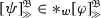iff and .

Using Theorems 9 and 8 , and our results for ranking and belief-revision semantics, we obtain completeness results for ${{\,\mathrm{\gg }\,}}$ in these alternative semantics:

Corollary 2

${{\,\mathrm{\gg }\,}}$ defined as sufficient reason in the semantics on the left (or >-logic in the middle) has the sound and complete ${{\,\mathrm{\gg }\,}}$-logic on the right, as shown in Table 3.

Table 3 Completeness for Corollary 2. The semantics (on the left) with complete basic conditional logic (in the middle) has the complete sufficient reason logic on the right

Proof

By chaining our results. $\square$

The result also shows that the logic for the sufficient reason is the same in ranking semantics as in full belief revision models. Furthermore, contrary to a remark made by Spohn (2012, p. 118), the sufficient (and necessary) reason can be developed in belief revision semantics, as in other frameworks.

We can do the same for the necessary reason:

Example 5

(necessary reason) Let ${{\,\mathrm{\mathfrak {R}}\,}}$ and ${{\,\mathrm{\mathfrak {B}}\,}}$ as in Example 4. Truth for ${{\,\mathrm{\mathcal {L}}\,}}_{{{\,\mathrm{\ge }\,}}}$ in these models is denoted and and:

$6^{{{\,\mathrm{\mathfrak {R}}\,}}}_{{{\,\mathrm{\ge }\,}}}$.:

iff .

$6^{{{\,\mathrm{\mathfrak {B}}\,}}}_{{{\,\mathrm{\ge }\,}}}$.:

iff and .

Again, by chaining, we get:

Corollary 3

${{\,\mathrm{\ge }\,}}$ defined as necessary reason in the semantics on the left (or >-logic in the middle) has the sound and complete ${{\,\mathrm{\ge }\,}}$-logic on the right, as shown in Table 4.

Table 4 Completeness for Corollary 3. The semantics (on the left) with complete basic conditional logic (in the middle) has the complete necessary reason logic on the right

This section showed that the sufficient and necessary reason relation can be developed in alternative semantics, illustrated by set-selection semantics, ranking semantics and belief revision semantics. Our method allowed to transfer completeness and soundness results to these settings. Other alternative semantics, for which there is a completeness result or for which such a result can easily be figured out, can be treated similarly. For example, ${{\mathsf {V}}}$ is also sound and complete for Leitgeb’s (2012) Popper measure semantics and thus the sufficient and necessary reason can be developed there—their logic is the same as for Lewisean models.

10 Conclusion

This article laid out a general technique to transfer completeness results of a known basic conditional > to a definable conditional ${{\,\mathrm{\vartriangleright }\,}}$. The technique was implemented for the sufficient reason $\varphi {{\,\mathrm{\gg }\,}}\psi := (\varphi> \psi ) \wedge \lnot (\lnot \varphi > \psi )$ and the necessary reason $\varphi {{\,\mathrm{\ge }\,}}\psi := (\lnot \varphi> \lnot \psi ) \wedge \lnot (\varphi > \lnot \psi )$ in a neighbourhood selection semantics, where > complies with a slightly augmented classical conditional logic. The technique generalises point equivalence lifted to classes. For this reason, we could also transfer the results to alternative stronger semantics, here exemplified with set selection semantics, ranking semantics and belief revision semantics. The technique could be applied equally to the weaker probabilistic threshold semantics of Hawthorne (2014).

Other definable conditionals can be treated by the same method. For example, the following conditional constructions (modulo translation):

• $\varphi {{\,\mathrm{{{\,\mathrm{\Diamond }\,}}\rightarrow }\,}}\psi := \lnot (\varphi {{\,\mathrm{{{\,\mathrm{\square }\,}}\rightarrow }\,}}\lnot \psi )$ (dual)

• $\varphi {{\,\mathrm{\blacktriangleright }\,}}\psi : = (\varphi> \psi ) \wedge \lnot (\varphi > \bot )$ (neutral)

• $\varphi {{\,\mathrm{\succ }\,}}\psi := (\varphi> \psi ) \wedge (\lnot \varphi > \lnot \psi )$ (dependency)

• $\varphi {{\,\mathrm{\vartriangleright }\,}}\psi := (\varphi> \psi ) \wedge (\lnot \psi > \lnot \varphi )$ (evidential)

The backdefinition (modulo backtranslation) would be¹⁷:

• $\varphi {{\,\mathrm{{{\,\mathrm{\square }\,}}\rightarrow }\,}}\psi := \lnot (\varphi {{\,\mathrm{{{\,\mathrm{\Diamond }\,}}\rightarrow }\,}}\lnot \psi )$ (dual)

• $\varphi > \psi := (\varphi {{\,\mathrm{\blacktriangleright }\,}}\psi ) \vee \lnot (\varphi {{\,\mathrm{\blacktriangleright }\,}}\top )$ (neutral)

• $\varphi > \psi := \varphi {{\,\mathrm{\succ }\,}}(\varphi \wedge \psi )$ (dependency)

• $\varphi > \psi := (\varphi \wedge \psi ) \vee (\varphi {{\,\mathrm{\vartriangleright }\,}}(\varphi \wedge \psi ))$ (evidential)

where these are respectively well behaved in minimal models, rcm-cn minimal models, rcm-cn-wcc minimal models, and for the evidential conditional one needs at least to add Lewis’ centering assumptions.

The theory was developed in a minimal logic and in a flexible semantics for the basic conditional. One could thus further transfer to many other alternative semantics. In particular, the above mentioned conditionals cover specific conditionals developed in stronger semantics: Lewis’ (1973b) dual conditional (${{\,\mathrm{{{\,\mathrm{\Diamond }\,}}\rightarrow }\,}}$, where the basic conditional ${{\,\mathrm{{{\,\mathrm{\square }\,}}\rightarrow }\,}}$ has at least logic ${{\mathsf {V}}}$), Lewis’ (1973a) counterfactual dependency (${{\,\mathrm{\succ }\,}}$, for > with logic ${{\mathsf {V}}}$), Spohn’s (2012) sufficient and necessary reason (${{\,\mathrm{\gg }\,}}$ and ${{\,\mathrm{\ge }\,}}$, for > with logic ${{\mathsf {VP}}}$), Rott’s (2019) difference making and dependency conditional (${{\,\mathrm{\gg }\,}}$ and ${{\,\mathrm{\succ }\,}}$, for > with logic ${{\mathsf {AGM}}}$ or ${{\mathsf {VP}}}$), Raidl’s (2019) neutral conditional (${{\,\mathrm{\blacktriangleright }\,}}$, for > with logic ${{\mathsf {V}}}$ or ${{\mathsf {VP}}}$) or the similar possibilistic conditional of Benferhat et al. (1997), as well as Crupi and Iacona’s (2019) evidential conditional (${{\,\mathrm{\vartriangleright }\,}}$, for > with logic ${{\mathsf {VC}}}$).

The theory can also be extended to languages containing additional modals or more than one conditional. For example, to treat conditional constructions of the following type (modulo translation):

• (doxastic)

• (metaphysic)

• (disjunctive)

• (simple)

A backdefinition (modulo backtranslation) of into the language with > and $\boxminus$ is¹⁸:

• (doxastic)

I analysed the doxastic and metaphysic conditional in ranking semantics (Raidl 2019), where $\boxminus$ is an S5 necessity. In fact, both are disjunctive conditionals. The counterpossible conditional of Berto et al. (2018) could also be analysed as a disjunctive conditional, with $>_1$ the neutral conditional ${{\,\mathrm{\blacktriangleright }\,}}$ and $>_2$ a conditional which satisfies no conditional law, apart from $(\varphi >_2 \varphi )$. The simple or ‘relevance’-conditional was analysed by Casini et al. (2019), where $>_1$ and $>_2$ have the logic ${{\mathsf {CE}}} + {{\mathsf {Cm}}}$. And the list probably continues. The hope is indeed, that more complex conditional constructions could be treated, such as Spohn’s (2015) supererogatory reason, or the probabilistic-causal conditional of van Rooij and Schulz (2019).

The neutral, doxastic, metaphysic and counterpossible conditionals were devised to treat the problem of vacuously true conditionals with impossible antecedent. The sufficient reason, the dependency, the evidential, the simple and the probabilistic-causal conditional were devised to capture relevance. Comparing the logics of these conditionals, also allows to test these new conditionals against possible counter-examples within the context for which they were developed.

Our investigation shows that the study of conditionals is not as messy as it might appear at first glance. Many conditional constructions can be obtained as definable conditionals from a basic conditional. As a consequence, many conditional constructions which attempt to solve one or the other problem of the Lewis–Stalnaker account by strengthening or weakening the basic conditional, can be analysed in a uniform fashion. The basic conditional constitutes a shared nucleus. And I would like to close with a conjecture: The strengthenings or weakenings of that nucleus are contextually variable and express implicit presuppositions. The nucleus however, represents a psychological, linguistic or conceptual constant.

References

Benferhat S, Dubois D, Prade H (1997) Nonmonotonic reasoning, conditional objects and possibility theory. Artif Intell 92:259–276
Berto F, French R, Priest G, Ripley D (2018) Williamson on coun-terpossibles. J Philos Logic 47(4):693–713
Casini G, Meyer T, Varzinczak I (2019) Simple conditionals with constrained right weakening. In: Proceedings of the twenty-eighth international joint conference on artificial intelligence, IJCAI-19, p 16321638
Chellas BF (1975) Basic conditional logic. J Philos Logic 4(2):133–153
Crupi V, Iacona A (2019) The evidential conditional. Preprint http://philsci-archive.pitt.edu/16759/
Friedman N, Halpern JY (2001) Plausibility measures and default reasoning. J ACM 48(4):648–685
Gärdenfors P (1986) Belief revisions and the ramsey test for conditionals. Philos Rev 95(1):81–93
Hawthorne J (2014) New Horn rules for probabilistic consequence: Is O\(+\) enough? In: Hansson SO (ed) David Makinson on classical methods for non-classical problems. Springer, Dordrecht, pp 157–166
Kraus S, Lehmann DJ, Magidor M (1990) Nonmonotonic reasoning, preferential models and cumulative logics. Artif Intell 44(1):167–207
Krzyżanowska K, Wenmackers S, Douven I (2013) Inferential conditionals and evidentiality. J Logic Lang Inf 22(3):315–334
Leitgeb H (2012) A probabilistic semantics for counterfactuals. Part A. Rev Symb Logic 5(1):26–84
Lewis D (1971) Completeness and decidability of three logics of counterfactual conditionals. Theoria 37(1):74–85
Lewis D (1973a) Causation. J Philos 70(17):556–567
Lewis D (1973b) Counterfactuals. Blackwell, Oxford
Raidl E (2018) Ranking semantics for doxastic necessities and conditionals. In: Arazim P, Lávička T (eds) The logica yearbook 2017. College Publications, Norcross, pp 223–238
Raidl E (2019) Completeness for counter-doxa conditionals—using ranking semantics. Rev Symb Logic 12(4):861–891
Rott H (2019) Difference-making conditionals and the relevant ramsey test. Rev Symb Logic 1–39: https://doi.org/10.1017/S1755020319000674
Skovgaard-Olsen N (2016) Motivating the relevance approach to conditionals. Mind Lang 31(5):555–579
Spohn W (2012) The laws of belief. Oxford University Press, Oxford
Spohn W (2015) Conditionals: a unifying ranking-theoretic perspective. Philos’ Imprint 15(1):1–30
Stalnaker RC (1968) A theory of conditionals. In: Rescher N (ed) Studies in logical theory (American philosophical quarterly monographs 2). Blackwell, Oxford, pp 98–112
van Rooij R, Schulz K (2019) Conditionals, causality and conditional probability. J Logic Lang Inf 28(1):55–71
Acknowledgements
Open access funding provided by Projekt DEAL. I would like to thank an anonymous referee who has significantly contributed to improving the readability of the paper. I first tested these ideas at the Dagstuhl Seminar 19032 and I thank the working group “The semantics of conditionals”, especially Gabriele Kern-Isberner and Mario Günther, for their enthusiasm. I also thank the people present at BRAON’19. I would particularly like to thank André Fuhrmann, Hans Rott, and Niels Skovgaard-Olsen for discussions, as well as Vincenzo Crupi and Andrea Iacona—exchanging with them helped me simplify important parts of the initial material.
Author information
Authors and Affiliations
Corresponding author
Additional information
This research was funded by the Deutsche Forschungsgemeinschaft (DFG, German Research Foundation) under Research Unit FOR 1614, and under Germany’s Excellence Strategy by the DFG Cluster of Excellence “Machine Learning: New Perspectives for Science”, EXC-Number 2064/1, Project number 390727645.
Rights and permissions
Open Access This article is licensed under a Creative Commons Attribution 4.0 International License, which permits use, sharing, adaptation, distribution and reproduction in any medium or format, as long as you give appropriate credit to the original author(s) and the source, provide a link to the Creative Commons licence, and indicate if changes were made. The images or other third party material in this article are included in the article’s Creative Commons licence, unless indicated otherwise in a credit line to the material. If material is not included in the article’s Creative Commons licence and your intended use is not permitted by statutory regulation or exceeds the permitted use, you will need to obtain permission directly from the copyright holder. To view a copy of this licence, visit http://creativecommons.org/licenses/by/4.0/.
About this article
Cite this article
Raidl, E. Definable Conditionals. Topoi 40, 87–105 (2021). https://doi.org/10.1007/s11245-020-09704-3
Published:
Issue Date:
DOI: https://doi.org/10.1007/s11245-020-09704-3